A posteriori error estimation for coarse or distorted meshes

Franz Chouly^∗

Michel Duprez^†

Claudio Lobos^‡

Zuqi Tang^§

Abstract

Finite element simulations carried out on meshes issued from real-world geometries — patient-specific anatomies, scanned industrial parts, fractured media — almost never satisfy the shape-regularity assumptions under which classical a posteriori error analysis is written. Practitioners are therefore left without a quantitative answer to a very legitimate question: how wrong is my simulation when my mesh is coarse and contains badly shaped elements?

In this work, we study to which extent equilibrated flux estimators can provide such an answer. Indeed, they deliver a guaranteed and fully computable upper bound of the energy-norm discretization error, with a constant equal to one; and, crucially for the present study, its derivation uses no shape-regularity, quasi-uniformity or angle condition. The only geometric ingredient is the Poincaré constant on a single cell, which Payne and Weinberger showed to be at most $h_{K} / π$ on any convex cell $K,$ however distorted $(h_{K}$ being the cell size). Mesh quality affects the local efficiency — the sharpness of the estimator — but never its reliability, so that the failure mode under distortion is pessimism rather than false confidence.

We study the case of conforming Lagrange finite element methods: the analysis is written for general cells in two and three space dimensions, and the numerical experiments are carried out with simplicial elements in two dimensions. We detail two flux reconstructions — a global $H (div)$ mixed one and the patchwise one (in the spirit of works from Braess and Schöberl or Ern and Vohralík) — and we map the geometric quality measures used by the meshing community onto the constants that do, and do not, appear in the analysis. The estimator is then assessed numerically on families of coarse, locally damaged, anisotropic and globally distorted meshes, against the residual, Zienkiewicz–Zhu-type recovery and Bank–Weiser estimators, and a duality argument extends the guarantee to a quantity of interest.

Across the $49$ computations reported here — including meshes of a letter glyph produced by two independent meshers, one of which ships with a zero-area cell — the guaranteed bound never failed, while the recovery estimator reported less error than was committed in every run on a mesh of the unit square. The Bank–Weiser estimator is sharper on every well-shaped mesh, but a single needle cell out of two thousand costs it a factor of $2. 6,$ and it falls below the true error on the L-shaped domain, where nothing in its output signals the failure. The two reconstructions of the guaranteed bound are found to degrade under different distortions: the global one under global anisotropy, the patchwise one under an accumulation of flattened cells within a single patch.

Keywords. a posteriori error estimation; distorted meshes; equilibrated fluxes; finite element method; guaranteed error bounds; mesh quality.

Mathematics Subject Classification. 65N15, 65N30, 65N50.

1 Introduction

In an idealised numerical analysis paper, the mesh is a parameter of the method: it is refined at will, it is shape-regular, and asymptotic statements in mesh size $h$ are meaningful. In a large part of engineering and biomedical practice, the situation is reversed: the mesh is a datum. It is produced by an automatic mesher from a segmented medical image, from a CAD model with slivers, or from a geometry containing thin features and cracks; it is as coarse as the computing budget allows; and it contains a small (or not so small) number of elements that any quality criterion would reject. Remeshing may be impossible (the geometry is not available any more), or undesirable (the mesh carries material data, or is the output of a registration procedure as in, e.g., [BLP10, Lob13]).

The question addressed here is therefore not how to build a better mesh, but rather: given this mesh and this solution, what is the guaranteed accuracy of the computed quantity? Any answer that involves an unspecified generic constant $C$ — as is the case for the classical explicit residual estimator — is of little practical use, and any answer whose validity is conditioned on a shape-regularity parameter is precisely useless in the regime we target, since that parameter blows up. What is wanted is a number that is computable from the data at hand, that is an upper bound with no hidden constant, and whose derivation does not quietly assume the mesh to be good.

A posteriori error estimation.

A posteriori error estimation started with Babuška and Rheinboldt [BR78]; the literature is now vast, and we refer to the monographs of Ainsworth and Oden [AO00], Verfürth [Ver13], Repin [Rep08], to the survey of Nochetto, Siebert and Veeser [NSV09] for the adaptive side, and to the lecture notes of Vohralík [Voh20], which we follow closely in Section 7.

Equilibrated flux estimators are based on ideas from Prager–Synge [PS47] and early contributions date back to the pioneering work of Ladèveze [LL83, LP04]; later contributions include Destuynder–Métivet [DM99], Luce–Wohlmuth [LW04], Braess–Schöberl [BS08, BPS09], Ern–Vohralík [EV15, EV20], Carstensen–Merdon [CM13, CM14], Becker–Capatina–Luce [BCL16], all of which give a guaranteed bound with constant one. Their common root is convex duality and the primal–dual gap: see Repin [Rep00, Rep08], Han [Han05], and, more recently and in a much broader nonsmooth setting, Bartels and Kaltenbach [BK23]. We come back to this reading in Remark 7.5. Fully computable bounds of residual type also exist, at the price of a careful tracking of the interpolation constants: see Veeser and Verfürth [VV09] and Carstensen and Merdon [CMN13, CM14]. Those constants still depend on the element shapes, which is exactly what we want to avoid here.

Finite elements on bad meshes.

On the a priori side, it is classical since Babuška and Aziz [BA76] that the minimum angle condition can be replaced by a maximum angle condition in 2D, and by suitable variants in 3D [Kří92]; anisotropic interpolation theory [Ape99, FP01, Pic03] pushes this further. Duprez, Lleras and Lozinski [DLL19] showed that a locally damaged mesh — a few arbitrarily distorted cells in an otherwise regular mesh — does not spoil the convergence rate, nor irreparably the conditioning.

Mesh quality measures.

The meshing community quantifies element quality through geometric or algebraic measures: aspect ratio, minimum/maximum dihedral angle, (scaled) Jacobian, condition number of the Jacobian, mean ratio, and their many variants; see the monograph of Frey and George [FG08], the algebraic framework of Knupp [Knu01] and the discussion of Shewchuk [She02] on which of those measures actually control interpolation error and conditioning. One contribution of the present work is to connect these practical measures with the constants that appear (and, more importantly, with those that do not appear) in the equilibrated flux analysis.

1.1 Contributions and outline

We revisit the equilibrated flux framework with an explicit tracking of the diffusion parameter $μ$ and of every geometric assumption used in the derivation of the upper bound (Sections 2–7). We isolate the single place where geometry enters — the Poincaré constant on a cell, Lemma 7.7 — and we explain how to keep the bound guaranteed on non-convex cells.
We review the geometric quality measures used in meshing and map them onto the constants of the analysis (Section 6), distinguishing between what affects the guarantee (almost nothing) and what affects the efficiency (a lot).
We describe two flux reconstructions (Sections 7.4 and 7.5): a global mixed one, in which the flux is sought in a Raviart–Thomas or Brezzi–Douglas–Marini subspace of $H (div, Ω)$ over the whole mesh, expensive but trivial to implement, and the patchwise one of Braess–Schöberl / Ern–Vohralík, cheap and parallel, and we discuss the practical pitfalls on distorted cells. Both are implemented, and Section 10.8 shows that they are not interchangeable under distortion: they lose sharpness under different geometric defects.
We compare with the residual, Zienkiewicz–Zhu-type recovery and Bank–Weiser estimators (Section 8) and quantify how each of them degrades with distortion. The comparison with Bank–Weiser (Section 10.10) is the substantive one: it is the sharper estimator on any mesh one would choose, and the more fragile on any mesh one would not choose.
We extend the guaranteed bound to a quantity of interest via a duality argument (Section 9), and we verify numerically that the resulting product bound is also insensitive to an isolated degenerate cell (Section 10.13).
We report numerical experiments (Section 10) on families of coarse, damaged, anisotropic and globally distorted meshes, and on the real meshes mentioned above. All the code is available and every table and figure in the paper is regenerated by it.

What is, and what is not, new.

None of the theory of Section 7 is new: the hypercircle identity is due to Prager and Synge [PS47], the relaxation to cellwise equilibration and the patchwise reconstruction are due to Vohralík and coworkers [Voh20, EV15] and to Braess and Schöberl [BS08]. What we claim is a change of reading. The absence of any shape-regularity hypothesis in the upper bound is, in that literature, a technical remark; here it is the object of the study, and we track it deliberately — isolating the one geometric ingredient that does appear (Lemma 7.7), stating what breaks when it fails (Remark 7.8), and measuring, rather than asserting, how much sharpness distortion actually costs. The mapping between the quality measures that meshing software reports and the constants that the analysis contains (Section 6) is, to our knowledge, not written down anywhere. The experimental observations of Section 10 — that the two reconstructions of the same guaranteed bound degrade under different defects, that Bank–Weiser is sensitive to a collapsed edge and not to a collapsed area, and that no single quality measure of Definition 6.1 predicts the local effectivity — are, likewise, new.

Scope.

We restrict ourselves to the Poisson problem with a piecewise constant coefficient, to conforming Lagrange elements, and — in the experiments — to two space dimensions and low order piecewise linear finite element approximation. These choices are motivated by the following. The phenomenon we want to isolate is geometric, and every additional feature of the model would make it harder to attribute an effect to the mesh alone. The consequences of relaxing each of these restrictions are discussed in Section 11. We also do not address the algebraic error: all linear systems below are solved by a direct method.

2 Notation

Let $Ω \subset R^{d},$ $d \in {2, 3},$ be a bounded Lipschitz polytopal domain with boundary $Γ : = \partial Ω .$ For $ω \subseteq Ω$ we write ${(\cdot, \cdot)}_{ω}$ for the $L^{2} (ω)$ scalar product (as well as for its vector-valued counterpart) and $‖ \cdot ‖_{ω}$ for the associated norm; the subscript is dropped when $ω = Ω .$ We use the standard Sobolev spaces $H^{1} (Ω),$ $V : = H_{0}^{1} (Ω),$ and

H (div, Ω) : = {τ \in [L^{2} (Ω)]^{d} : div τ \in L^{2} (Ω)} .

For $τ \in H (div, Ω)$ and $v \in V,$ the Green formula

\begin{array}{cr} {(τ, \nabla v)}_{Ω} + {(div τ, v)}_{Ω} = 0 & (1) \end{array}

holds (the boundary term vanishes since $v$ has zero trace).

3 Model problem

Let $μ > 0$ be a physical parameter, assumed piecewise constant on the mesh introduced below, and let $f \in L^{2} (Ω) .$ We consider the Poisson problem with homogeneous Dirichlet boundary conditions:

\begin{array}{cr} - d i v (μ \nabla u) = f in Ω, u = 0 on Γ . & (2) \end{array}

Define the bilinear and linear forms

\begin{array}{cr} a (v, w) : = {(μ \nabla v, \nabla w)}_{Ω}, ℓ (v) : = {(f, v)}_{Ω}, v, w \in V, & (3) \end{array}

so that the weak formulation reads: find $u \in V$ such that

\begin{array}{cr} a (u, v) = ℓ (v), \forall v \in V . & (4) \end{array}

By Lax–Milgram, (4) is well posed. We measure the error in the energy norm

\begin{array}{cr} | | | v | | | : = ‖ μ^{1 / 2} \nabla v ‖_{Ω}, | | | v | | |_{ω} : = ‖ μ^{1 / 2} \nabla v ‖_{ω}, & (5) \end{array}

and we associate with it the dual norm on fluxes, $‖ μ^{- 1 / 2} τ ‖_{ω} .$ The exact flux is

\begin{array}{cr} σ : = - μ \nabla u \in H (div, Ω), div σ = f in Ω . & (6) \end{array}

4 The mesh

Let $T_{h}$ be a partition of $\overset{―}{Ω}$ into closed cells $K$ with $\overset{―}{Ω} = ⋃_{K \in T_{h}} K$ and $\overset{˚}{K} \cap \overset{˚}{K^{'}} = \emptyset$ for $K / = K^{'} .$ We assume only that $T_{h}$ is

Assumption 4.1 (Admissible mesh).

(M1) matching: the intersection of two distinct cells is either empty, or a common vertex, edge or face (no hanging node)¹.
(M2) each cell $K$ is the image of a fixed reference cell $\hat{K}$ (simplex, quadrilateral/hexahedron, prism, . . . ) by a smooth, invertible map $F_{K} : \hat{K} \to K$ with $\det (J_{K}) > 0$ everywhere on $\hat{K},$ where $J_{K} : = D F_{K};$
(M3) $μ$ is constant on each $K,$ with value $μ_{K} .$

We stress what is not assumed: no shape regularity $(h_{K} / ρ_{K} \leq γ,$ with $ρ_{K}$ the inradius), no quasi-uniformity $(\max_{K} h_{K} / \min_{K} h_{K} \leq γ),$ no minimum nor maximum angle condition, no bound on the number of cells sharing a vertex, no convexity of the cells. The mesh may be a simplicial one, a tensor-product one, or a mixed one.

We write $h_{K} : = diam (K),$ $h : = \max_{K \in T_{h}} h_{K},$ and $F_{h}$ for the set of faces, split into interior faces $F_{h}^{i}$ and boundary faces $F_{h}^{b} .$ The set of vertices is $V_{h} = V_{h}^{i} \cup V_{h}^{b}$ (interior / boundary). For a vertex $a \in V_{h},$ $ω_{a}$ denotes the patch of cells sharing $a$ and $ψ_{a}$ the associated $P_{1}$ hat function $(supp ψ_{a} = ω_{a},$ $\sum_{a} ψ_{a} \equiv 1).$ For a cell $K,$ $ω_{K} : = ⋃ {ω_{a} : a \in K} .$

5 The finite element method

Let $k \geq 1$ and let

\begin{array}{cr} V_{h} : = {v_{h} \in V : v_{h} \circ F_{K} \in P_{k} (\hat{K}) \forall K \in T_{h}} \subset V & (7) \end{array}

be the conforming Lagrange finite element space $(Q_{k}$ on tensor-product cells); we refer to [Bra07, EG21] for the general theory. The discrete problem reads: find $u_{h} \in V_{h}$ such that

\begin{array}{cr} a (u_{h}, v_{h}) = ℓ (v_{h}), \forall v_{h} \in V_{h} . & (8) \end{array}

Conformity $V_{h} \subset V$ gives Galerkin orthogonality

\begin{array}{cr} a (u - u_{h}, v_{h}) = 0, \forall v_{h} \in V_{h}, & (9) \end{array}

which we will use twice: to obtain the Prager–Synge identity, and — crucially — to guarantee the solvability of the local Neumann problems of Section 7.5.

Remark 5.1 (Conformity). Because $V_{h} \subset V,$ no potential reconstruction is needed and the framework of [Voh20, EV15] simplifies to a flux reconstruction only. For nonconforming, DG or mixed discretizations, the estimator gains a nonconformity term; see [EV15].

6 Measuring the quality of a mesh

This section collects the quality measures that a mesher produces, and confronts them with the constants of the a posteriori analysis. Throughout, $J_{K} (\hat{x}) = D F_{K} (\hat{x}) \in R^{d \times d}$ denotes the Jacobian matrix of the geometric map at $\hat{x} \in \hat{K},$ with singular values

ς_{1} (K) \geq \cdot \cdot \cdot \geq ς_{d} (K) > 0.

6.1 Geometric and algebraic quality measures

Definition 6.1 (Usual quality measures). For a cell $K$ we consider

(Q1) the shape-regularity ratio $γ_{K} : = h_{K} / ρ_{K},$ $ρ_{K}$ being the diameter of the largest ball inscribed in $K;$
(Q2) the aspect ratio $α_{K} : = ς_{1} (K) / ς_{d} (K),$ i.e. the condition number of $J_{K}$ in the spectral norm (for triangles we take $\hat{K}$ equilateral here, so that $α_{K} = 1$ characterises the equilateral cell and the value does not depend on the numbering of the vertices);
(Q3) the scaled Jacobian $s_{K} : = \min_{\hat{x}} [\det (J_{K} (\hat{x})) / \prod_{i = 1}^{d} ‖ (J_{K} (\hat{x}))_{:, i} ‖_{2}] \in [- 1, 1]$ equal to $1$ when the columns of $J_{K}$ are orthogonal and tending to $0$ for a flat (sliver, cap, needle) element, and negative for an inverted one, i.e. one whose vertices are traversed in the wrong orientation ( $\det (J_{K}) < 0),$ which (M2) excludes. For a triangle the bracket is the sine of the angle at the vertex onto which $F_{K}$ maps the origin of $\hat{K};$ to make the measure independent of the numbering of the vertices we take, as mesh-quality software does, its minimum over the three corners, $s_{K} = \min_{i} \sin θ_{i} (K),$ $θ_{i} (K)$ being the angles of $K .$ This equals $1 / \sqrt{2} \approx 0.71$ on the right triangles of a structured mesh (the value $s_{\min}$ reported for family (F1) in Section 10), $\sqrt{3} / 2$ on the equilateral triangle, and is of order $t$ for both the needle and the cap of family (F3);
(Q4) the Frobenius condition number $κ_{K} : = \frac{1}{d} ‖ J_{K} ‖_{F} ‖ J_{K}^{- 1} ‖_{F} \geq 1$ and the associated mean ratio $1 / κ_{K}$ [Knu01];
(Q5) the extremal angles $θ_{\min} (K),$ $θ_{\max} (K)$ (dihedral angles in 3D).

These measures are not equivalent, and the differences matter. In 2D, a triangle family with $θ_{\max} \to π$ (cap) and one with $θ_{\min} \to 0$ but $θ_{\max}$ bounded away from $π$ (needle) both have $γ_{K} \to \infty,$ but only the first one destroys the $H^{1}$ interpolation error [BA76, She02]. This is a first hint that the classical shape-regularity ratio (Q1) is a crude proxy.

6.2 Where does geometry enter the analysis?

Let us anticipate on Section 7 and list the constants involved.

(C1) Poincaré constant on a cell. The upper bound uses
$‖ φ - {\overset{―}{φ}}_{K} ‖_{K} \leq C_{P, K} h_{K} ‖ \nabla φ ‖_{K}, φ \in H^{1} (K),$
where ${\overset{―}{φ}}_{K}$ is the mean value of $φ$ over $K .$ By Payne–Weinberger [PW60], $C_{P, K} \leq 1 / π$ for any convex $K,$ regardless of its shape — a needle, a sliver or a cap triangle all admit $C_{P, K} = 1 / π,$ and no better uniform value is available since $1 / π$ is attained in the limit of a thin slab. This is the reason why the guaranteed bound survives distortion. Convexity is however essential: for a non-convex cell the constant need not be $1 / π$ (see Remark 7.8).
(C2) Cauchy–Schwarz. Used several times, constant one, no geometry.
(C3) Local equilibration solvability. Involves only Galerkin orthogonality (9) and the partition of unity, no geometry.
(C4) Efficiency (lower bound). The bound $η_{K} ≲ | | | u - u_{h} | | |_{ω_{K}} + {osc}_{K}$ relies on bubble-function / discrete stability arguments whose constants do degenerate with $γ_{K},$ with $α_{K},$ and with the number of cells in a patch [EV15, BPS09].
(C5) Conditioning and a priori error. Not the subject here, but recall that the condition number of the stiffness matrix and the interpolation constants degrade with $α_{K}$ and $θ_{\max}$ [She02, DLL19].

The message is summarised in Table 1.


	guaranteed	efficiency	cost
	upper bound	(lower bound)
Explicit residual	no (unknown $C)$	degenerates	cheap
Fully computable residual [VV09, CM14]	yes, $C$ shape-dependent	degenerates	cheap
Zienkiewicz–Zhu [ZZ87]	no	asympt. exact	very cheap
		if regular
Bank–Weiser [BW85, BHL⁺23]	under saturation	degenerates	moderate
Equilibrated flux	yes, $C = 1,$	degenerates	moderate
	geometry-free

Table 1: Sensitivity of the main estimator families to the mesh quality. Only the sharpness of the equilibrated flux estimator is affected by distortion; its reliability is not.

6.3 A quality field to be correlated with the estimator

For the numerical section we define, for each cell, the vector of quality indicators

\begin{array}{cr} q_{K} : = (γ_{K}, α_{K}, s_{K}, κ_{K}, θ_{\min} (K), θ_{\max} (K)), & (10) \end{array}

and we will study the empirical correlation between $q_{K}$ and the local effectivity index

\begin{array}{cr} I_{K} : = \frac{η_{K}}{| | | u - u_{h} | | |_{ω_{K}}}, η_{K} : = η_{K}^{F} + η_{K}^{R}, & (11) \end{array}

the local indicators $η_{K}^{F},$ $η_{K}^{R}$ being defined in (18)–(17) below.

The claim to be tested is that the global effectivity index (24) stays $O (1)$ under distortion for the equilibrated flux estimator, whereas its residual and Zienkiewicz–Zhu counterparts drift — and, in the case of the latter, drifts below one, which is the dangerous direction.

7 A posteriori error estimation

We now come to the a posteriori error estimates. The guiding thread is the equilibrated flux methodology: it is the only one, among those recalled in Section 8, whose upper bound is both fully computable and free of any assumption on the geometry of the cells.

7.1 The Prager–Synge identity

Definition 7.1 (Admissible flux). A vector field $p$ is admissible for (2) if

\begin{array}{cr} p \in H (div, Ω) and div p = f in Ω . & (AC) \end{array}

Theorem 7.2 (Prager–Synge [PS47]). Let $u \in V$ solve (4), let $p$ satisfy (AC) and let $v \in V$ be arbitrary. Then

\begin{array}{cr} ‖ μ^{- 1 / 2} (p + μ \nabla v) ‖^{2} = ‖ μ^{- 1 / 2} (p - σ) ‖^{2} + | | | u - v | | |^{2} . & (12) \end{array}

Proof. Write $p + μ \nabla v = (p - σ) + μ \nabla (v - u),$ using $σ = - μ \nabla u .$ Expanding the square,

‖ μ^{- 1 / 2} (p + μ \nabla v) ‖^{2} = ‖ μ^{- 1 / 2} (p - σ) ‖^{2} + | | | u - v | | |^{2} + 2 (p - σ, \nabla (v - u)) .

Set $w : = v - u \in V .$ By (1) and (AC), $(p, \nabla w) = - (div p, w) = - (f, w),$ while by (4), $(- σ, \nabla w) = (μ \nabla u, \nabla w) = a (u, w) = (f, w) .$ The two contributions cancel, which is the orthogonality property at the heart of the identity. □

Corollary 7.3 (Hypercircle bound). Taking $v = u_{h}$ in (12) and dropping the first term on the right,

\begin{array}{cr} | | | u - u_{h} | | | \leq \inf_{p satisfying (AC)} ‖ μ^{- 1 / 2} (p + μ \nabla u_{h}) ‖ . & (13) \end{array}

Three features of (13) deserve emphasis, and they are the reason for this work:

the multiplicative constant is one: this is a true, quantitative bound on the error, not an asymptotic statement;
every admissible $p$ gives a valid bound, so the estimator is a certificate that can be checked a posteriori;
nothing in the proof involves the mesh — in fact no mesh is needed at all, which suggests that the same machinery applies to meshless or immersed methods.

The difficulty is of course that (AC) is an equality of functions in $L^{2} (Ω),$ and building a discrete field that satisfies it exactly for a general $f$ is out of reach in practice. The next subsection removes this obstruction.

Before doing so, we record the convex-duality reading of (12), which explains why the constant is one.

Proposition 7.4 (The estimator is a primal–dual gap). Define the primal and dual (complementary) energies

\begin{array}{cr} E (v) : = \frac{1}{2} a (v, v) - ℓ (v), v \in V, E^{*} (p) : = - \frac{1}{2} ‖ μ^{- 1 / 2} p ‖^{2}, p satisfying (AC) . & (14) \end{array}

Then $\min_{v \in V} E (v) = E (u) = E^{*} (σ) = \max_{p} E^{*} (p)$ — there is no duality gap — and, for every $v \in V$ and every admissible $p,$

\begin{array}{cr} E (v) - E^{*} (p) = \frac{1}{2} | | | u - v | | |^{2} + \frac{1}{2} ‖ μ^{- 1 / 2} (p - σ) ‖^{2} = \frac{1}{2} ‖ μ^{- 1 / 2} (p + μ \nabla v) ‖^{2} . & (15) \end{array}

Proof. Since $a (u, v) = ℓ (v),$ one has $E (v) = \frac{1}{2} a (v - u, v - u) - \frac{1}{2} a (u, u) = \frac{1}{2} | | | u - v | | |^{2} - \frac{1}{2} ‖ μ^{1 / 2} \nabla u ‖^{2} .$ On the other hand, for $p$ admissible, (1) and (4) give $(μ^{- 1} p, σ) = - (p, \nabla u) = (div p, u) = (f, u) = ‖ μ^{1 / 2} \nabla u ‖^{2},$ whence

\frac{1}{2} ‖ μ^{- 1 / 2} (p - σ) ‖^{2} = \frac{1}{2} ‖ μ^{- 1 / 2} p ‖^{2} - ‖ μ^{1 / 2} \nabla u ‖^{2} + \frac{1}{2} ‖ μ^{- 1 / 2} σ ‖^{2} = - E^{*} (p) - \frac{1}{2} ‖ μ^{1 / 2} \nabla u ‖^{2},

using $‖ μ^{- 1 / 2} σ ‖ = ‖ μ^{1 / 2} \nabla u ‖ .$ Adding the two displays gives the first equality in (15); the second one is Theorem 7.2. Taking $v = u$ and $p = σ$ shows that the gap vanishes, and non-negativity of (15) gives weak duality. □

Remark 7.5 (Duality reading of the hypercircle). Proposition 7.4 says that the squared estimator $‖ μ^{- 1 / 2} (σ_{h} + μ \nabla u_{h}) ‖^{2}$ is nothing but twice the primal–dual gap evaluated at the computed pair $(u_{h}, σ_{h}) :$ it is a by-product of weak duality, which holds for any admissible pair and involves no discretization whatsoever. This is why the constant is one, and this is the viewpoint — a posteriori estimation by duality — underlying the functional error estimates of Repin [Rep00, Rep08] and Han [Han05]; Bartels and Kaltenbach [BK23] have recently extended it to general convex minimisation, including nonsmooth and degenerate problems, where the quadratic structure used above is unavailable.

7.2 The abstract framework of Vohralík: relaxing the admissibility condition

Following [Voh20, Chap. 7] and [EV15] we only require equilibration in the mean on each cell.

Definition 7.6 (Equilibrated flux reconstruction). A field $σ_{h}$ is an equilibrated flux reconstruction if

\begin{array}{cr} σ_{h} \in H (div, Ω) and {(div σ_{h} - f, 1)}_{K} = 0 \forall K \in T_{h} . & (EF) \end{array}

Lemma 7.7 (Poincaré on a cell). Let $K$ be a convex cell and $φ \in H^{1} (K)$ with mean value ${\overset{―}{φ}}_{K} .$ Then

\begin{array}{cr} ‖ φ - {\overset{―}{φ}}_{K} ‖_{K} \leq \frac{h_{K}}{π} ‖ \nabla φ ‖_{K} . & (16) \end{array}

Proof. This is the Payne–Weinberger inequality [PW60]; the constant $h_{K} / π$ is optimal (attained in the limit of a thin rectangle/cylinder) and depends on $K$ only through its diameter. □

Remark 7.8 (Non-convex cells). Inequality (16) may fail on a non-convex cell. Three remedies keep the bound guaranteed: (i) split each non-convex cell into convex sub-cells for the purpose of evaluating $η_{K}^{R}$ only, and use $h_{K^{'}} / π$ on each sub-cell $K^{'}$ — this only improves the estimate since $h_{K^{'}} \leq h_{K};$ (ii) use the constant $C_{P, K} h_{K}$ with $C_{P, K}$ computed from a local eigenvalue problem (a small, purely local computation); (iii) when $f$ is a piecewise polynomial of degree at most $p,$ make the term vanish by using a reconstruction with $div σ_{h} = Π_{p} f,$ see Proposition 7.12; for a general $f$ the data oscillation (22) remains and still involves the Poincaré constant of the cell. In our numerical experiments all cells are triangles, hence convex, and Lemma 7.7 applies directly; the reconstructions used there satisfy $div σ_{h} = Π_{p} f$ exactly, so that $η_{K}^{R}$ reduces to the data oscillation (22).

We now define the two families of local indicators, for each $K \in T_{h} :$

\begin{aligned} η_{K}^{R} & : = \frac{h_{K}}{π} μ_{K}^{- 1 / 2} ‖ f - div σ_{h} ‖_{K} & (residual, or equilibration defect, indicator) & (17) \\ η_{K}^{F} & : = ‖ μ^{- 1 / 2} (σ_{h} + μ \nabla u_{h}) ‖_{K} & (flux, or constitutive relation, indicator) . & (18) \end{aligned}

Both are computable once $u_{h}$ and $σ_{h}$ are at hand: they involve no unknown constant and no reference to the exact solution.

Theorem 7.9 (Guaranteed upper bound). Let $u$ solve (4), $u_{h}$ solve (8), and let $σ_{h}$ satisfy (EF). Assume the cells are convex (see Remark 7.8 otherwise). Then

\begin{array}{cr} | | | u - u_{h} | | |^{2} \leq \sum_{K \in T_{h}} {(η_{K}^{R} + η_{K}^{F})}^{2} = : η^{2} . & (19) \end{array}

Proof. Since $u - u_{h} \in V,$ and by definition of the energy norm,

\begin{array}{cr} | | | u - u_{h} | | | = \sup_{φ \in V, | | | φ | | | = 1} a (u - u_{h}, φ) . & (20) \end{array}

Fix such a $φ .$ Using (4),

a (u - u_{h}, φ) = (f, φ) - (μ \nabla u_{h}, \nabla φ) .

Insert $\pm div σ_{h}$ and use the Green formula (1) for $σ_{h} \in H (div, Ω)$ and $φ \in V,$ i.e. $(div σ_{h}, φ) = - (σ_{h}, \nabla φ) :$

\begin{array}{cr} a (u - u_{h}, φ) = \underset{= : T_{R}}{\underset{⏟}{(f - div σ_{h}, φ)}} \underset{= : T_{F}}{\underset{⏟}{- (σ_{h} + μ \nabla u_{h}, \nabla φ)}} . & (21) \end{array}

For $T_{F},$ a cellwise Cauchy–Schwarz inequality gives

T_{F} \leq \sum_{K \in T_{h}} ‖ μ^{- 1 / 2} (σ_{h} + μ \nabla u_{h}) ‖_{K} ‖ μ^{1 / 2} \nabla φ ‖_{K} = \sum_{K \in T_{h}} η_{K}^{F} | | | φ | | |_{K} .

For $T_{R},$ split over the cells and use (EF) to subtract the cell mean of $φ$ for free:

T_{R} = \sum_{K \in T_{h}} {(f - div σ_{h}, φ)}_{K} = \sum_{K \in T_{h}} {(f - div σ_{h}, φ - {\overset{―}{φ}}_{K})}_{K} .

Cauchy–Schwarz and Lemma 7.7 then yield

\begin{aligned} T_{R} & \leq \sum_{K \in T_{h}} ‖ f - div σ_{h} ‖_{K} \frac{h_{K}}{π} ‖ \nabla φ ‖_{K} \\ = \sum_{K \in T_{h}} [\frac{h_{K}}{π} μ_{K}^{- 1 / 2} ‖ f - div σ_{h} ‖_{K}] [μ_{K}^{1 / 2} ‖ \nabla φ ‖_{K}] = \sum_{K \in T_{h}} η_{K}^{R} | | | φ | | |_{K}, \end{aligned}

where we inserted $1 = μ_{K}^{- 1 / 2} μ_{K}^{1 / 2},$ licit because $μ$ is constant on $K$ by (M3). Summing the two bounds and applying a last, discrete Cauchy–Schwarz inequality,

a (u - u_{h}, φ) \leq \sum_{K \in T_{h}} (η_{K}^{R} + η_{K}^{F}) | | | φ | | |_{K} \leq (\sum_{K \in T_{h}} (η_{K}^{R} + η_{K}^{F})^{2})^{1 / 2} (\sum_{K \in T_{h}} | | | φ | | |_{K}^{2})^{1 / 2},

Remark 7.10 (What was not used). The proof used: the conformity $V_{h} \subset V$ (through $u - u_{h} \in V),$ the $H (div) -$ conformity of $σ_{h}$ (through the Green formula), the cellwise equilibration (EF), and the Poincaré inequality on convex cells. No shape regularity, no minimum/maximum angle, no quasi-uniformity, no bound on the patch cardinality, no asymptotic regime in $h .$ In particular (19) is valid on the coarsest and most distorted mesh, and even for $k = 1$ on a single element.

Remark 7.11 (Non-homogeneous Dirichlet data). Suppose $u = g$ on $Γ$ with $g$ in the trace space of $H^{1} (Ω),$ and let $u_{h} \in V_{h}$ satisfy (8) for all $v_{h} \in V_{h} \cap H_{0}^{1} (Ω)$ with its boundary values fixed to some $g_{h} .$ Theorem 7.9 goes through verbatim provided $u - u_{h} \in H_{0}^{1} (Ω),$ i.e. provided $g_{h} = g$ exactly on $Γ$ — the only place where the boundary condition entered the proof was through $u - u_{h} \in V$ and the vanishing of the boundary term in (1). If, as is usual, $g_{h}$ is merely an interpolant of $g,$ then $u - u_{h} / \in H_{0}^{1} (Ω)$ and an additional term appears, measuring the distance from $g_{h}$ to $g$ in $H^{1 / 2} (Γ);$ bounding it computably requires an argument of a different nature, and the constant it brings does depend on the shape of the boundary cells. This is why the main experiments of Section 10 are built on test cases with homogeneous Dirichlet data. The L-shaped test case (T2), whose exact solution $r^{2 / 3} \sin (2 θ / 3)$ has non-polynomial boundary values, therefore falls outside the theorem; we report it separately in Section 10.12 as an experiment on what happens when a hypothesis is dropped, not as evidence for the bound. This is a genuine gap in the theory presented here, not an oversight; see [EV15] for the treatment of general boundary data.

Proposition 7.12 (Data oscillation form). Assume the reconstruction satisfies the stronger property $div σ_{h} = Π_{p} f,$ where $Π_{p}$ denotes the $L^{2} -$ orthogonal projection onto the space of piecewise polynomials of degree at most $p$ (broken, i.e. cellwise). Then $η_{K}^{R}$ reduces to the data oscillation

\begin{array}{cr} {osc}_{K} (f) : = \frac{h_{K}}{π} μ_{K}^{- 1 / 2} ‖ f - Π_{p} f ‖_{K}, & (22) \end{array}

which is exactly computable, involves neither $u_{h}$ nor $σ_{h},$ and is of order $h_{K}^{p + 2}$ on each cell where $f \in H^{p + 1} (K)$ — at least one order better than $η_{K}^{F},$ which is of order $h^{k},$ as soon as $p \geq k - 1 .$ It vanishes identically when $f$ is itself a piecewise polynomial of degree $\leq p .$

Remark 7.13 (When may the residual term be dropped?). Only under the hypothesis of Proposition 7.12, and even then it should be computed rather than dropped, since it is cheap. For a reconstruction that merely satisfies (EF), $η_{K}^{R}$ is of the same order as $η_{K}^{F}$ and neglecting it destroys the guarantee. Classical presentations are often silent on this distinction; the FEniCS script of Section 10.2 evaluates both terms.

7.3 Efficiency, and where the mesh quality strikes back

Reliability is the good news; efficiency is where geometry returns. We state the known result informally, as we shall not use it quantitatively.

Theorem 7.14 (Local efficiency [BPS09, EV15, EV20, CZ12]). For the patchwise reconstruction of Section 7.5 on a simplicial mesh, there holds

\begin{array}{cr} η_{K}^{F} \leq C_{s t} (γ_{ω_{K}}) (| | | u - u_{h} | | |_{ω_{K}} + {osc}_{ω_{K}} (f)), {osc}_{ω_{K}} (f)^{2} : = \sum_{K^{'} \subset ω_{K}} {osc}_{K^{'}} (f)^{2}, & (23) \end{array}

where $C_{s t}$ depends on the shape-regularity $γ_{ω_{K}} : = \max_{K^{'} \subset ω_{K}} γ_{K^{'}}$ of the patch and on its cardinality, but neither on the polynomial degree $k,$ which is the content of [BPS09, EV20], nor on the diffusion contrast, which for conforming elements is the result of Cai and Zhang [CZ12], obtained without any quasi-monotonicity assumption on $μ .$

Combining Theorems 7.9 and 7.14, the effectivity index

\begin{array}{cr} I : = \frac{η}{| | | u - u_{h} | | |} & (24) \end{array}

satisfies $1 \leq I \leq C_{s t} (γ)$ up to oscillation: the lower bound $I \geq 1$ is unconditional, whereas the upper bound degrades with the mesh quality. Distortion can therefore make the estimator pessimistic, never unreliable. From an engineering standpoint this is exactly the right failure mode — the user is never told that the solution is more accurate than it is. Quantifying the growth of $I$ with the quality vector (10) is one of the objectives of Section 10.

Remark 7.15 (Locally damaged meshes). Following [DLL19], if only a small subset $T_{h}^{d a m} \subset T_{h}$ of cells is distorted, one expects $C_{s t}$ to degrade only on the patches touching $T_{h}^{d a m},$ so that the global effectivity index remains $O (1) :$ the few bad patches contribute a bounded amount to the sum. The relevant parameter should then be the diameter of the damaged patch, not the quality of an isolated cell. This is a conjecture we probe numerically in Section 10.6.

7.4 A first (expensive) estimator: global mixed $H (div)$ formulation

We now describe two ways of producing a $σ_{h}$ satisfying (EF). The first, presented here, is trivial to implement and expensive; the second, Section 7.5, is the method of choice. Fix $p \geq 0$ and let

\begin{array}{cr} Q_{h} : = {q_{h} \in L^{2} (Ω) : q_{h} |_{K} \in P_{p} (K) \forall K \in T_{h}}, V_{h} \subset H (div, Ω) with div V_{h} = Q_{h} . & (25) \end{array}

Admissible choices on a simplicial mesh are the Raviart–Thomas pair $V_{h} = {R T}_{p} (T_{h})$ [RT77] and the Brezzi–Douglas–Marini pair $V_{h} = {B D M}_{p + 1} (T_{h})$ [BDM85]. The degree shift matters: $div {R T}_{q} = P_{q}$ because ${R T}_{q} = [P_{q}]^{d} \oplus x {\tilde{P}}_{q},$ whereas ${B D M}_{q} = [P_{q}]^{d}$ only gives $div {B D M}_{q} = P_{q - 1};$ pairing ${B D M}_{p}$ with $P_{p}$ would be unstable. Both pairs above are inf-sup stable [BBF13]. We then solve the dual mixed formulation of (2): find $(σ_{h}, λ_{h}) \in V_{h} \times Q_{h}$ such that

\begin{array}{cr} {\begin{aligned} {(μ^{- 1} σ_{h}, τ_{h})}_{Ω} - {(λ_{h}, div τ_{h})}_{Ω} & = 0 & \forall τ_{h} \in V_{h}, \\ {(div σ_{h}, q_{h})}_{Ω} & = {(f, q_{h})}_{Ω} & \forall q_{h} \in Q_{h} . \end{aligned} & (26) \end{array}

Since $div V_{h} = Q_{h},$ the second equation is equivalent to $div σ_{h} = Π_{p} f;$ hence (EF) holds exactly, up to round-off, and Proposition 7.12 applies. The first equation is the weak form of the constitutive relation $μ^{- 1} σ + \nabla λ = 0$ — the Dirichlet condition $u = 0$ being natural here, it is enforced weakly and no essential constraint is imposed on $V_{h} .$ Thus $λ_{h}$ approximates $u$ and $σ_{h}$ approximates the exact flux $σ = - μ \nabla u$ directly in $H (div, Ω);$ see [CM13] for the analysis of the resulting estimator.

Remark 7.16 (Pros and cons). Pros: three lines of FEniCS/FreeFEM, no local solver to write, and it produces an exactly equilibrated flux. Cons: it requires the solution of a global saddle-point problem, typically more expensive than the primal problem it is supposed to certify, which defeats the purpose in a production run. It is however perfect as a reference implementation, and this is how we use it in Section 10.

Remark 7.17 (Do not simply project the discrete flux). A tempting shortcut is to take $σ_{h} : = Π_{V_{h}} (- μ \nabla u_{h}),$ the $L^{2} -$ projection of the discrete flux onto ${R T}_{p} .$ The result does belong to $H (div, Ω),$ so the Green formula used in Theorem 7.9 is still valid, and the bound (19) still holds. But nothing forces (EF), so $η_{K}^{R}$ is no longer a data oscillation: it is a genuine term of the same order as $η_{K}^{F},$ and the bound, though valid, becomes useless in practice. Such a projection is essentially a Zienkiewicz–Zhu recovery in disguise (Section 8); the whole point of an equilibrated reconstruction is precisely to make the residual term collapse to (22).

7.5 Patchwise reconstruction (Braess–Schöberl / Ern–Vohralík)

The efficient construction localises (26) on vertex patches, using the partition of unity $\sum_{a \in V_{h}} ψ_{a} = 1 .$ The idea is to build separately, on each patch, an approximation of the localised exact flux $ψ_{a} σ,$ and to sum them up. The divergence of that target is, by the Leibniz rule and (6),

\begin{array}{cr} div (ψ_{a} σ) = ψ_{a} div σ + \nabla ψ_{a} \cdot σ = ψ_{a} f - μ \nabla u \cdot \nabla ψ_{a}, & (27) \end{array}

which dictates the local right-hand side below — note the minus sign, which is what makes the local Neumann problem compatible.

For $a \in V_{h},$ set

\begin{array}{cr} \begin{aligned} V_{h}^{a} & : = {τ_{h} \in {R T}_{p} (ω_{a}) : τ_{h} \cdot n = 0 on \partial ω_{a} ∖ Γ}, \\ Q_{h}^{a} & : = {q_{h} \in L^{2} (ω_{a}) : q_{h} |_{K} \in P_{p} (K) \forall K \subset ω_{a}, and {(q_{h}, 1)}_{ω_{a}} = 0 if a \in V_{h}^{i}}, \end{aligned} & (28) \end{array}

so that $div V_{h}^{a} = Q_{h}^{a} .$ The zero-mean constraint on $Q_{h}^{a},$ and the homogeneous normal trace on the whole of $\partial ω_{a}$ that goes with it, reflect the pure Neumann nature of the local problem at an interior vertex; at a boundary vertex the normal trace is left free on $\partial ω_{a} \cap Γ$ and no mean-value constraint is needed. Solve, for each $a,$ the local mixed problem: find $(σ_{h}^{a}, r_{h}^{a}) \in V_{h}^{a} \times Q_{h}^{a}$ such that

\begin{array}{cr} {\begin{aligned} {(μ^{- 1} σ_{h}^{a}, τ_{h})}_{ω_{a}} - {(r_{h}^{a}, div τ_{h})}_{ω_{a}} & = - {(ψ_{a} \nabla u_{h}, τ_{h})}_{ω_{a}} & \forall τ_{h} \in V_{h}^{a}, \\ {(div σ_{h}^{a}, q_{h})}_{ω_{a}} & = {(g_{a}, q_{h})}_{ω_{a}} & \forall q_{h} \in Q_{h}^{a}, \end{aligned} & (29) \end{array}

with the local right-hand side suggested by (27),

\begin{array}{cr} g_{a} : = ψ_{a} f - μ \nabla u_{h} \cdot \nabla ψ_{a} . & (30) \end{array}

Note that the factor $μ^{- 1}$ in the first equation of (29) cancels the factor $μ$ carried by the target $- ψ_{a} μ \nabla u_{h},$ which is why $μ$ does not appear on its right-hand side. Equivalently, and this is the form to keep in mind, $σ_{h}^{a}$ is the constrained minimiser

\begin{array}{cr} σ_{h}^{a} = \arg \min_{\begin{matrix} τ_{h} \in V_{h}^{a} \\ div τ_{h} = Π_{p} g_{a} \end{matrix}} ‖ μ^{- 1 / 2} (τ_{h} + ψ_{a} μ \nabla u_{h}) ‖_{ω_{a}}, & (31) \end{array}

i.e. the equilibrated field closest, in the $μ^{- 1} -$ weighted $L^{2}$ norm, to the localised discrete flux $- ψ_{a} μ \nabla u_{h};$ here $r_{h}^{a}$ is the Lagrange multiplier of the divergence constraint. Finally set

\begin{array}{cr} σ_{h} : = \sum_{a \in V_{h}} σ_{h}^{a}, & (32) \end{array}

each $σ_{h}^{a}$ being extended by zero outside $ω_{a} .$

Proposition 7.18 (The construction is well posed and equilibrated). Let $k \geq 1,$ so that $ψ_{a} \in V_{h}$ (see [EV15] for the choice of $p$ as a function of $k).$ Then:

(i) For $a \in V_{h}^{i},$ problem (29) is well posed. Indeed, the pure Neumann compatibility condition ${(g_{a}, 1)}_{ω_{a}} = 0$ required for $Π_{p} g_{a}$ to belong to $div V_{h}^{a} = Q_{h}^{a}$ reads
${(g_{a}, 1)}_{ω_{a}} = {(f, ψ_{a})}_{Ω} - {(μ \nabla u_{h}, \nabla ψ_{a})}_{Ω} = ℓ (ψ_{a}) - a (u_{h}, ψ_{a}) = 0,$
which is exactly the discrete problem (8) tested with the hat function $ψ_{a} \in V_{h} .$ This is where the minus sign in (30) is essential: with a plus sign one would obtain $2 ℓ (ψ_{a}) / = 0$ and the local problem would have no solution.
(ii) Each $σ_{h}^{a}$ has zero normal trace on $\partial ω_{a} ∖ Γ,$ so its extension by zero has no normal jump across $\partial ω_{a}$ and belongs to $H (div, Ω);$ hence so does the finite sum $σ_{h} .$
(iii) $div σ_{h}^{a} = Π_{p} g_{a}$ on $ω_{a} .$ For a boundary vertex this is immediate since $Q_{h}^{a}$ is the full broken polynomial space. For an interior vertex, the second equation of (29) only gives that $div σ_{h}^{a} - Π_{p} g_{a}$ is $L^{2} -$ orthogonal to all zero-mean $q_{h},$ i.e. is a constant $c$ on $ω_{a};$ but ${(div σ_{h}^{a}, 1)}_{ω_{a}} = \int_{\partial ω_{a}} σ_{h}^{a} \cdot n = 0 = {(Π_{p} g_{a}, 1)}_{ω_{a}}$ by (i), so $c = 0 .$
(iv) Consequently, using $\sum_{a} ψ_{a} \equiv 1$ and hence $\sum_{a} \nabla ψ_{a} \equiv 0,$
$div σ_{h} = \sum_{a} Π_{p} g_{a} = Π_{p} (f \sum_{a} ψ_{a} - μ \nabla u_{h} \cdot \sum_{a} \nabla ψ_{a}) = Π_{p} f .$
Therefore (EF) holds and Proposition 7.12 applies: the residual indicator reduces to the data oscillation (22).

The whole procedure is summarised as follows.

Algorithm 7.19 (Guaranteed error bound, patchwise version).

Solve the primal problem (8) for $u_{h} .$
For each vertex $a \in V_{h}$ (in parallel): assemble $g_{a}$ by (30) and solve the local mixed problem (29) for $σ_{h}^{a} .$
Assemble $σ_{h} : = \sum_{a} σ_{h}^{a}$ by (32).
Certificate check (cheap, optional but recommended): verify that $\max_{K} | {(div σ_{h} - f, 1)}_{K} |$ is at round-off level.
For each cell $K,$ evaluate $η_{K}^{F}$ by (18) and $η_{K}^{R} = {osc}_{K} (f)$ by (22).
Return $η = (\sum_{K} (η_{K}^{R} + η_{K}^{F})^{2})^{1 / 2} .$ By Theorem 7.9, $| | | u - u_{h} | | | \leq η,$ whatever the mesh.

Remark 7.20 (Cost and parallelism). Step 2 requires $# V_{h}$ independent mixed solves, each of a size depending only on $p$ and on the number of cells in the patch, and each independent of the others: the step is embarrassingly parallel and its complexity is linear in $# V_{h},$ against a global saddle-point solve for the reconstruction of Section 7.4. On the meshes of Section 10 with $k = 1$ and $p = 1,$ each local system has at most $43$ unknowns, so the arithmetic cost of step 2 is a few hundred flops per vertex. We report that algebraic size rather than a wall-clock comparison: our driver loops over the patches in Python, and its running time measures the interpreter, not the algorithm (Section 10.8).

Remark 7.21 (The correction term of the classical constructions). An alternative and historically earlier route (Destuynder–Métivet [DM99], Ladèveze [LP04]) is to build a first field ${\tilde{p}}_{h} : = \sum_{a} p_{h}^{a}$ that equilibrates only approximately, and then to add a cellwise correction $δ p_{K},$ obtained by solving a local Neumann problem on $K,$ so that $p_{h} |_{K} : = {\tilde{p}}_{h} |_{K} + δ p_{K}$ is exactly admissible. The subtlety, easily overlooked, is that the correction must be computed exactly for the bound to remain guaranteed; if it is computed in a finite dimensional space, it is not exactly admissible, and one is back to the relaxed setting of Definition 7.6. Presentations that assert that the correction is “negligible” implicitly assume a fine and shape-regular mesh — which is precisely the assumption we do not make. The formulation (29) sidesteps the issue altogether: the constraint $div τ_{h} = Π_{p} g_{a}$ is imposed inside the discrete space, and the residual defect is exactly the computable oscillation of Proposition 7.12.

Remark 7.22 (Distorted cells: implementation pitfalls). On strongly distorted or nearly degenerate cells the local matrices in (29) become badly conditioned. Practical remedies: (i) scale the $R T$ basis by the face measures; (ii) solve (31) in the constrained least-squares form with an orthonormalised basis of the divergence constraint; (iii) use a direct solver with pivoting on each patch — the matrices are tiny. Note that a badly conditioned local problem does not compromise the guarantee: any computed $σ_{h}$ that lies in $H (div, Ω)$ and passes the check ${(div σ_{h} - f, 1)}_{K} = 0$ (verifiable a posteriori, to round-off) gives a valid bound, however suboptimal. Note also that the approximation properties of the ${R T}_{p}$ interpolant on strongly anisotropic tetrahedra are known and better than the isotropic theory suggests [AADL11], which is encouraging for the anisotropic mesh family (F5) below.

8 Comparison with other estimators

8.1 Explicit residual

The classical explicit residual estimator reads, on a simplicial mesh,

\begin{array}{cr} η_{K}^{r e s} : = (C_{1}^{2} h_{K}^{2} μ_{K}^{- 1} ‖ f + d i v (μ \nabla u_{h}) ‖_{K}^{2} + C_{2}^{2} \sum_{F \subset \partial K \cap F_{h}^{i}} h_{F} μ_{F}^{- 1} ‖ [[μ \nabla u_{h} \cdot n]] ‖_{F}^{2})^{1 / 2}, & (33) \end{array}

where $[[\cdot]]_{F}$ is the jump across the face $F,$ $h_{F} : = diam F,$ $μ_{F}$ the larger of the two adjacent values of $μ,$ and $C_{1}, C_{2}$ are fixed normalisation constants. One has $| | | u - u_{h} | | | \leq C (\sum_{K} (η_{K}^{r e s})^{2})^{1 / 2}$ with $C$ depending on the shape-regularity of $T_{h}$ through the constants of the Clément [Clé75] / Scott–Zhang [SZ90] quasi-interpolation; see [BMV01, Ver13] for a careful discussion. Two defects, both fatal in our context: $C$ is not computable, and $C \to \infty$ as the elements degenerate (for a triangle, $C$ grows like $(\sin θ_{\max})^{- 1}$ or worse). Fully computable variants [VV09, CM14] replace $C$ by an explicit expression, which however still involves the element shapes. We nevertheless include $η^{r e s}$ in the comparison, with the usual engineering choice $C = 1,$ precisely to exhibit its unreliability on distorted meshes.

8.2 Recovery estimators of Zienkiewicz–Zhu type

With $G_{h} : [L^{2}]^{d} \to [V_{h}]^{d}$ a gradient recovery operator (patch averaging, superconvergent patch recovery, . . . ),

\begin{array}{cr} η_{K}^{Z Z} : = ‖ μ^{1 / 2} (G_{h} (\nabla u_{h}) - \nabla u_{h}) ‖_{K} . & (34) \end{array}

Cheap, popular, asymptotically exact on structured shape-regular meshes thanks to superconvergence [ZZ92a, ZZ92b] — and with no guarantee whatsoever otherwise. The variant implemented below takes for $G_{h}$ the global $L^{2} -$ projection of $\nabla u_{h}$ onto the continuous $[P_{1}]^{d}$ space, the simplest member of the family; it is not the superconvergent patch recovery of [ZZ92a, ZZ92b], and the superscript “ZZ” used throughout is a shorthand for the recovery principle, not for that particular smoothing. Superconvergence is exactly the property that a distorted mesh destroys, so $η^{Z Z}$ is expected to be the least robust of the four; anisotropic variants exist [Pic03].

8.3 Bank–Weiser

This is the closest competitor of the equilibrated flux estimator, and the one we shall follow quantitatively throughout Section 10: like the patchwise reconstruction of Section 7.5 it solves small local problems, and it is the estimator with the reputation of being the sharpest.

The Bank–Weiser estimator [BW85] solves one local Neumann-type problem per cell. Let

\begin{array}{cr} V_{K}^{B W} : = {v \in P_{k + 1} (K) : v (a) = 0 \forall a \in V_{h} \cap K}, & (35) \end{array}

which for $k = 1$ is the three-dimensional span of the quadratic edge bubbles, i.e. $P_{2} (K)$ modulo $P_{1} (K)$ in the hierarchical sense; see [BHL⁺23] for the systematic construction at arbitrary $k$ and its FEniCS implementation. Find $e_{K}^{B W} \in V_{K}^{B W}$ with

\begin{array}{cr} {(μ \nabla e_{K}^{B W}, \nabla v)}_{K} = {(f + div (μ \nabla u_{h}), v)}_{K} - \frac{1}{2} \sum_{F \subset \partial K \cap F_{h}^{i}} {([[μ \nabla u_{h} \cdot n]], v)}_{F} \forall v \in V_{K}^{B W}, & (36) \end{array}

and set $η_{K}^{B W} : = | | | e_{K}^{B W} | | |_{K} .$ The right-hand side is the residual functional $ℓ (v) - a (u_{h}, v)$ written cellwise, each facet integral being split half and half between its two cells. Four remarks, which are what the numerical comparison will put figures on.

(a) No boundary condition is imposed on $V_{K}^{B W} :$ since the space contains no constant, the local bilinear form is already positive definite on it, and the pure Neumann problem (36) is solvable without any compatibility condition. This is what makes Bank–Weiser cheap, and it is also the reason it needs no equilibration step — and gets no guarantee in exchange.
(b) Reliability holds only under a saturation assumption — that the $P_{k + 1}$ solution be strictly closer to $u$ than the $P_{k}$ one by a fixed factor. The resulting constant is not one, it depends on the shape regularity, and, unlike the equilibration defect of step 4 of Algorithm 7.19, the assumption cannot be checked a posteriori: nothing in the computed output tells the user whether the bound holds.
(c) The $1 / 2$ split of the facet term is the classical, unweighted choice, and it is not robust with respect to the diffusion coefficient: the jump $[[μ \nabla u_{h} \cdot n]]$ carries the larger of the two values of $μ,$ while the local form on the low-coefficient side weighs it against the smaller one. Coefficient-weighted splits repair this; we use the classical version, and Section 10.10 shows what it costs.
(d) Cost: (36) is symmetric positive definite and of dimension $\dim P_{k + 1} (K) - # {vertices}$ — three for $k = 1$ in 2D — against a saddle-point problem over a whole vertex patch for the equilibrated reconstruction. Per local solve, Bank–Weiser is the cheaper of the two.

8.4 Summary

Table 1 summarises the situation. The point we want to make is not that the equilibrated flux estimator is the sharpest. It is not: on the finest structured mesh of Table 2 Bank–Weiser overestimates by $0.4 %$ where the equilibrated flux overestimates by $0.8 %,$ and on the under-resolved boundary layer it is sharper still $(1 .74$ against $2.4 0).$ The point is that it is the only one of the four whose validity does not evaporate when the mesh is bad — and, as Section 10.10 shows, the sharpness advantage of Bank–Weiser is exactly what distortion takes away.

9 Goal-oriented estimation

Engineers rarely care about the energy norm; they care about a quantity of interest $J (u)$ — a displacement at a point, a flux through a surface, an average stress. Let $J \in V^{'}$ be a bounded linear functional and let $z \in V$ solve the dual problem

\begin{array}{cr} a (v, z) = J (v) \forall v \in V, & (37) \end{array}

approximated by $z_{h} \in V_{h}$ with $a (v_{h}, z_{h}) = J (v_{h})$ for all $v_{h} \in V_{h} .$

Proposition 9.1 (Guaranteed goal-oriented bound). There holds

\begin{array}{cr} | J (u) - J (u_{h}) | = | a (u - u_{h}, z - z_{h}) | \leq | | | u - u_{h} | | | | | | z - z_{h} | | | \leq η^{p r i m} η^{d u a l}, & (38) \end{array}

where $η^{p r i m}$ and $η^{d u a l}$ are the equilibrated flux estimators (19) of the primal and of the dual problem.

Proof. $J (u) - J (u_{h}) = a (u - u_{h}, z)$ by (37), and $a (u - u_{h}, z_{h}) = 0$ by Galerkin orthogonality (9), whence $J (u) - J (u_{h}) = a (u - u_{h}, z - z_{h}) .$ Conclude with the Cauchy–Schwarz inequality in the energy norm, then Theorem 7.9 applied twice. □

Again the constant is one and no mesh assumption is used. Since $a$ is symmetric, the dual problem is solved with the same stiffness matrix as the primal one — already factorised — so the extra cost is one additional right-hand side plus one additional flux reconstruction, that is, roughly a doubling of the estimation cost.

Two caveats are in order. First, (38) bounds $| J (u) - J (u_{h}) |$ but gives no information on its sign, whereas practice often calls for a signed correction; sharper, non-product bounds that also provide a lower bound are available [CNT23]. Second, the product form is pessimistic by construction, since it discards the cancellation between the primal and the dual error: the effectivity index of (38) grows like the ratio of the two error distributions. Section 10.13 quantifies this, and shows that the resulting index is nevertheless $O (1)$ and, like the energy bound itself, insensitive to an isolated degenerate cell.

10 Numerical experiments

All computations are performed with FEniCSx (dolfinx 0.9.0) in serial. All the scripts, meshes and raw result files are openly available at

https://github.com/michelduprez/A-posteriori-error-estimation-for-coarse-or-distorted-meshes

Every table and figure below is regenerated from that repository by a single driver, whose README documents the role of each file. Related open implementations are dolfin-tape [Ble16] and the Bank–Weiser code of [BHL⁺23].

10.1 Protocol

Test cases.

In each case the exact solution is known in closed form, so that the true error $| | | u - u_{h} | | |$ — and hence the effectivity index (24) — can be computed and the guarantee $η \geq | | | u - u_{h} | | |$ can be checked, not merely asserted.

(T1) Smooth: $Ω = (0, 1)^{2},$ $u (x) = \sin (π x_{1}) \sin (π x_{2}),$ $μ \equiv 1,$ $f = 2 μ π^{2} u,$ homogeneous Dirichlet data. Reference case: the error is smooth and equidistributed, so any deviation of $I$ from its structured-mesh value is attributable to the mesh alone.
(T2) Singular: L-shaped domain $Ω = (- 1, 1)^{2} ∖ ([0, 1] \times [- 1, 0]),$ $f = 0,$ and $u = r^{2 / 3} \sin (2 θ / 3),$ with $θ$ measured counter-clockwise from the positive $x_{1} -$ axis and running over $(0, 3 π / 2) .$ Here $u \in H^{1 + 2 / 3 - ϵ} (Ω)$ only, and the Dirichlet data are non-homogeneous on part of $\partial Ω,$ so that Theorem 7.9 does not apply verbatim (Remark 7.11). We run the case nevertheless, with $g_{h}$ the Lagrange interpolant of $g,$ precisely in order to see whether, and by how much, the bound fails; this is Section 10.12. It tests the estimator in the presence of a corner singularity, where the error is strongly localised.
(T3) Boundary layer: $Ω = (0, 1)^{2}$ and
$u (x) = (1 - e^{- x_{1} / ε}) (1 - e^{- (1 - x_{1}) / ε}) x_{2} (1 - x_{2}), ε = 10^{- 2},$
which vanishes on $\partial Ω$ and exhibits layers of width $ε$ near $x_{1} = 0$ and $x_{1} = 1;$ $f$ is obtained by differentiation. Natural companion of the anisotropic mesh family (F5).
(T4) Heterogeneous: $μ = 1$ for $x_{1} < 1 / 2$ and $μ = 10^{4}$ for $x_{1} > 1 / 2,$ with the interface aligned with the mesh as required by (M3). The interface is placed exactly where $\partial u / \partial x_{1} = 0$ for $u = \sin (π x_{1}) \sin (π x_{2}),$ so that the normal flux $μ \partial u / \partial x_{1}$ is continuous across it and this $u$ is the exact solution of the transmission problem, with $f = 2 μ π^{2} u \in L^{2} (Ω) .$ Checks the $μ -$ robustness announced in Theorem 7.9.

Mesh families.

The synthetic meshes (F1)–(F5) triangulate the unit square, so that the closed-form solutions above apply and the effectivity index can be measured rather than estimated; the real meshes (F6) and the L-shaped meshes (F7) do not, and are treated separately.

(F1) uniform structured meshes, $N = 8, . . ., 128$ (reference);
(F2) randomly perturbed meshes: every interior vertex is moved by $δ h ξ,$ $ξ$ uniform in the unit disc, $δ \in {0.10, 0.20, 0.30} .$ Since both endpoints of an edge move, the mesh stays untangled as long as $2 δ < 1 / \sqrt{2},$ i.e. $δ < 0.35 4;$ the code verifies a posteriori that no cell has been inverted;
(F3) locally damaged meshes: one single interior vertex is displaced, all other cells being left untouched, in the spirit of [DLL19]. Two variants, controlled by a parameter $t \in {10^{- 1}, . . ., 10^{- 4}} :$ needle, where the vertex is moved a fraction $1 - t$ of the way toward a neighbour (so $θ_{\min} \to 0$ while $θ_{\max}$ stays bounded away from $π,$ and the maximum angle condition still holds); and cap, where it is moved onto the opposite edge of one of its cells (so $θ_{\max} \to π$ and the maximum angle condition fails). In both cases $s_{K} \sim t;$
(F4) extent of the damage: $m \in {1, 4, 16, 64}$ vertices are cap-damaged at fixed $t = 1 0^{- 3},$ either scattered over the whole domain or grouped in a single contiguous block. At equal $m$ and equal local quality, the two layouts differ only by the diameter of the damaged region, which is precisely the parameter the conjecture of Section 7.3 points to. Damaged vertices are taken on the even sublattice so that no two of them are neighbours;
(F5) globally anisotropic structured meshes with $N \times M$ cells, $M \in {N, N / 4, N / 8, N / 16},$ hence aspect ratios up to $α \approx 1 6;$
(F6) the real meshes shipped with the project, treated separately in Section 10.15: a triangulation of $(- 1, 1)^{2}$ and four triangulations of a letter glyph, produced by two independent meshers;
(F7) structured triangulations of the L-shaped domain of (T2), with $2 N \times 2 N$ squares of side $1 / N$ over the enclosing square $(- 1, 1)^{2},$ each split into two right triangles and the cells of the missing quadrant removed, $N = 4, . . ., 3 2 .$ These are shape-regular meshes: they carry the singularity of (T2), not a geometric defect.

Figure 1 shows one representative of each synthetic family.

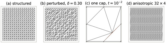
Figure 1: The synthetic mesh families. (a) the structured reference (F1); (b) the random perturbation (F2) at the largest admissible amplitude; (c) a zoom on the single cap-damaged vertex of (F3), the flattened cell being highlighted — every other cell of that mesh is the structured one of panel (a); (d) the anisotropic family (F5).

Quantities reported.

For each pair (test case, mesh) we report the true energy error $| | | u - u_{h} | | |,$ the four estimators, and their global effectivity indices (24). The equilibrated flux is computed with the ${B D M}_{1} \times P_{0}$ pair of Section 7.4; the residual estimator uses the engineering calibration $C_{1} = C_{2} = 1,$ and $G_{h}$ in (34) is the global $L^{2} -$ projection onto the continuous $[P_{1}]^{2}$ space. In addition we report

the certificate
$\max_{K} | {(div σ_{h} - f, 1)}_{K} | / \max {{(| f |, 1)}_{K}, {(| div σ_{h} |, 1)}_{K}, h_{K}^{- 1} {(| σ_{h} |, 1)}_{K}},$
which must be at round-off level (step 4 of Algorithm 7.19); the denominator is the size of the terms that must cancel, and does not degenerate when $f = 0$ as in test case (T2). It never exceeded $7.2 \cdot 10^{- 10}$ over the whole campaign, and $2.3 \cdot 10^{- 9}$ if the dual problems of Section 10.13 are included;
the worst cellwise ratio $η_{K} / | | | u - u_{h} | | |_{K}$ over the badly shaped cells $(s_{K} < 0. 1),$ written $I_{K}^{b a d} .$ Note that Theorem 7.14 bounds $η_{K}$ by the error on the patch $ω_{K},$ so a cellwise ratio slightly above one is expected and is not a violation of anything; the quantity is reported as a proxy for the local sharpness on the damaged cells.

10.2 How it is computed: a reference implementation

The listing below computes the equilibrated flux by the global mixed formulation (26) and evaluates both indicators (17) and (18), including the residual term that is often (wrongly) omitted, as well as the parameter $μ .$ It is a complete, runnable FEniCSx script; the output it produces is quoted after the listing.

Listing 1: Guaranteed error bound via a global ${B D M}_{1} \times P_{0}$ flux reconstruction. This is code/fenicsx/minimal_example.py included verbatim, so the listing and the script that produced the output below cannot drift apart.

from mpi4py import MPI
import numpy as np
import ufl
import basix.ufl
from dolfinx import fem, mesh as dmesh
from dolfinx.fem.petsc import LinearProblem

LU = {"ksp_type": "preonly", "pc_type": "lu",
      "pc_factor_mat_solver_type": "mumps"}
QD = {"quadrature_degree": 8}

# ------------------------------------------------------------ data ----
N = 64
mu = 1.0                            # physical parameter, tracked
msh = dmesh.create_unit_square(MPI.COMM_WORLD, N, N,
                              dmesh.CellType.triangle)

x = ufl.SpatialCoordinate(msh)
u_ex = ufl.sin(ufl.pi * x[0]) * ufl.sin(ufl.pi * x[1])
f = -ufl.div(mu * ufl.grad(u_ex))          # = 2 mu pi^2 u_ex

# -------------------------------------------------- primal problem ----
V = fem.functionspace(msh, ("Lagrange", 1))
msh.topology.create_connectivity(1, 2)
bdofs = fem.locate_dofs_topological(
    V, 1, dmesh.exterior_facet_indices(msh.topology))
bc = fem.dirichletbc(fem.Constant(msh, 0.0), bdofs, V)

u, v = ufl.TrialFunction(V), ufl.TestFunction(V)
uh = LinearProblem(ufl.inner(mu * ufl.grad(u), ufl.grad(v)) * ufl.dx(metadata=QD),
                   ufl.inner(f, v) * ufl.dx(metadata=QD),
                   bcs=[bc], petsc_options=LU).solve()

# ------------------------- equilibrated flux, global mixed ----
# Inf-sup stable pair BDM_{p+1} x P_p: div sigma_h = Pi_p f exactly.
p = 0
W = fem.functionspace(msh, basix.ufl.mixed_element([
    basix.ufl.element("BDM", msh.basix_cell(), p + 1),
    basix.ufl.element("DG", msh.basix_cell(), p)]))

(sig, lam) = ufl.TrialFunctions(W)
(tau, q) = ufl.TestFunctions(W)

#  ( mu^{-1} sigma_h , tau ) - ( lambda_h , div tau ) = 0
#  ( div sigma_h , q )                                = ( f , q )
# u = 0 is *natural* here: no essential boundary condition.
a = ((1.0 / mu) * ufl.inner(sig, tau) - lam * ufl.div(tau)
     + ufl.div(sig) * q) * ufl.dx(metadata=QD)
# f integrated with the same rule as in the certificate below: tested with
# q = 1_K, the second equation is then exactly the equilibration (EF).
L = ufl.inner(f, q) * ufl.dx(metadata=QD)
w = LinearProblem(a, L, bcs=[], petsc_options=LU).solve()
sig_h = w.sub(0)

# --------------------------------------------- cellwise indicators ----
DG0 = fem.functionspace(msh, ("DG", 0))
v0 = ufl.TestFunction(DG0)
dx = ufl.dx(metadata=QD)
h_K = ufl.CellDiameter(msh)


def cellwise(expr):
    return np.asarray(fem.assemble_vector(fem.form(expr * v0 * dx)).array)


r = sig_h + mu * ufl.grad(uh)
etaF = np.sqrt(cellwise((1.0 / mu) * ufl.inner(r, r)))       # eta_F
etaR = np.sqrt(cellwise((h_K / np.pi) ** 2 * (1.0 / mu)
                        * (f - ufl.div(sig_h)) ** 2))        # eta_R
eta = np.sqrt(((etaR + etaF) ** 2).sum())                    # bound

# ------------------------------------------------ check the bound ----
e = ufl.grad(uh - u_ex)
err = np.sqrt(fem.assemble_scalar(fem.form(ufl.inner(mu * e, e) * dx)))

# certificate: relative cellwise equilibration defect.  The scale is the
# largest of the terms that must cancel, so that the test stays meaningful
# when |f| is large -- and defined when f vanishes.
scale = np.maximum.reduce([cellwise(abs(f)), cellwise(abs(ufl.div(sig_h))),
                           cellwise(ufl.sqrt(ufl.inner(sig_h, sig_h)) / h_K)])
defect = np.abs(cellwise(ufl.div(sig_h) - f)) / scale

print(f"energy error   |||u-u_h|||   = {err:.6e}")
print(f"estimator      eta           = {eta:.6e}")
print(f"  flux part    ||etaF||      = {np.linalg.norm(etaF):.6e}")
print(f"  oscillation  ||etaR||      = {np.linalg.norm(etaR):.6e}")
print(f"effectivity    I = eta/err   = {eta / err:.4f}")
print(f"max rel. equilibration defect= {defect.max():.2e}")
assert eta >= err, "the guaranteed bound is violated -- check the code!"

Its output on the $64 \times 64$ mesh is

energy error   |||u-u_h|||   = 5.451370e-02
estimator      eta           = 5.539722e-02
  flux part    ||etaF||      = 5.450766e-02
  oscillation  ||etaR||      = 1.135797e-03
effectivity    I = eta/err   = 1.0162
max rel. equilibration defect= 1.03e-12

Three things are worth reading off these six lines. The bound holds with an effectivity of $1.6 %;$ the oscillation term (22) accounts for $2 %$ of the estimator, so it is small but not negligible — dropping it would give $η = 5.4508 \cdot 10^{- 2} < | | | u - u_{h} | | | = 5.4514 \cdot 10^{- 2}$ and the assertion on the last line would fire, which is exactly the trap of Remark 7.13; and the equilibration certificate is at round-off, so (EF) is verified to hold, and not merely assumed to.

The assertion on the last line is the central claim of the paper: it must never fire, whatever the mesh. Over the $32$ runs of the campaign that are covered by Theorem 7.9, and the one real mesh with a known solution, it never did — for either reconstruction. The patchwise variant of Section 7.5 replaces the global solve by $# V_{h}$ local ones; it is implemented in patchwise.py and reported in Section 10.8.

10.3 Reference case: convergence and asymptotic behaviour

Table 2 reports the reference family (F1) on the smooth test case (T1).


mesh	cells	$\| \| \| u - u_{h} \| \| \|$	$η^{e q}$	$I^{e q}$	$I^{B W}$	$I^{r e s}$	$I^{Z Z}$
F1 $N = 8$	128	4.318e-01	4.878e-01	1.130	1.082	5.526	0.960
F1 $N = 16$	512	2.175e-01	2.316e-01	1.065	1.037	5.601	0.984
F1 $N = 32$	2048	1.090e-01	1.125e-01	1.032	1.017	5.632	0.993
F1 $N = 64$	8192	5.451e-02	5.540e-02	1.016	1.008	5.645	0.997
F1 $N = 128$	32768	2.726e-02	2.748e-02	1.008	1.004	5.651	0.998

Table 2: Test case (T1) on the structured family (F1), $k = 1 .$ The equilibrated flux estimator is asymptotically exact $(I^{e q} \to 1),$ the residual estimator with $C = 1$ overestimates by a factor close to $5.6 5,$ and the recovery estimator converges to $1$ from below — it underestimates the error on every mesh of this family. Bank–Weiser is the sharpest of the four here, and stays above one.

Four observations, all of which persist throughout the campaign on the unit square.

$I^{e q}$ decreases monotonically from $1.130$ to $1.00 8 :$ the guaranteed bound is not merely valid, it becomes asymptotically exact. The residual indicator $η^{R}$ contributes only $‖ η^{R} ‖ / ‖ η^{F} ‖ \approx 2 %$ of the estimator at $N = 64$ and decreases at the higher rate predicted by Proposition 7.12.
$I^{r e s} \approx 5. 6 :$ the explicit residual estimator with the naive calibration $C = 1$ is off by more than half an order of magnitude. This is not a defect of the estimator but a reminder that its constant is unknown.
$I^{Z Z} < 1$ on every mesh. The recovery estimator underestimates the error — benignly here $(0 .96$ to $0.99 8),$ much less benignly below.
$I^{B W}$ is the sharpest of the four, $1.082$ down to $1.00 4 :$ on a structured mesh Bank–Weiser overestimates by about half as much as the equilibrated flux. Section 10.10 follows what becomes of that advantage.

10.4 Distorted meshes: the main experiment

Table 3 is the core of the paper: the same test case (T1) computed on meshes of steadily degrading quality.


mesh	$s_{\min}$	$θ_{\max}$ (deg)	$I^{e q}$	$I^{B W}$	$I^{r e s}$	$I^{Z Z}$	$I_{K}^{b a d}$
F2 $δ = 0.10$	5.6e-01	106.9	1.033	1.022	5.619	0.989	—
F2 $δ = 0.20$	4.0e-01	126.1	1.033	1.036	5.583	0.978	—
F2 $δ = 0.30$	2.3e-01	147.3	1.034	1.062	5.543	0.961	—
F3 needle $t = 10^{- 1}$	5.3e-02	132.0	1.032	1.021	5.637	0.992	1.00
F3 needle $t = 10^{- 2}$	5.0e-03	134.7	1.032	1.048	5.639	0.991	1.00
F3 needle $t = 10^{- 3}$	5.0e-04	135.0	1.032	1.282	5.640	0.991	1.00
F3 needle $t = 10^{- 4}$	5.0e-05	135.0	1.032	2.664	5.640	0.991	1.00
F3 cap $t = 10^{- 1}$	1.0e-01	168.6	1.032	1.023	5.631	0.992	1.00
F3 cap $t = 10^{- 2}$	1.0e-02	178.9	1.032	1.028	5.636	0.992	1.00
F3 cap $t = 10^{- 3}$	1.0e-03	179.9	1.032	1.028	5.637	0.992	1.00
F3 cap $t = 10^{- 4}$	1.0e-04	180.0	1.032	1.028	5.637	0.992	1.00
F4 scattered $m = 1$	1.0e-03	179.9	1.032	1.019	5.639	0.993	1.00
F4 block $m = 1$	1.0e-03	179.9	1.032	1.028	5.637	0.992	1.00
F4 scattered $m = 4$	1.0e-03	179.9	1.032	1.032	5.639	0.991	1.06
F4 block $m = 4$	1.0e-03	179.9	1.031	1.058	5.651	0.988	1.00
F4 scattered $m = 16$	1.0e-03	179.9	1.031	1.095	5.685	0.983	1.06
F4 block $m = 16$	1.0e-03	179.9	1.030	1.152	5.705	0.980	1.00
F4 scattered $m = 64$	1.0e-03	179.9	1.031	1.198	5.750	0.964	1.14
F4 block $m = 64$	1.0e-03	179.9	1.028	1.321	5.814	0.964	1.02
F5 $32 \times 32$	7.1e-01	90.0	1.032	1.017	5.632	0.993	—
F5 $32 \times 8$	2.4e-01	90.0	1.092	1.163	6.962	0.985	—
F5 $32 \times 4$	1.2e-01	90.0	1.182	1.529	8.648	0.965	—
F5 $32 \times 2$	6.2e-02	90.0	1.401	2.297	10.429	0.880	1.87

Table 3: Test case (T1), $N = 3 2,$ $k = 1,$ on the mesh families (F2)–(F5). The scaled Jacobian $s_{\min}$ degrades over four orders of magnitude and $θ_{\max}$ reaches $180$ degrees, yet $I^{e q}$ never leaves the interval $[1.028, 1.401]$ and is never below one. $I^{Z Z},$ by contrast, is below one in every single row, and $I^{B W}$ — the sharpest of the four on the structured mesh — reaches $2.664$ on the thinnest needle.

Figure 2 plots the same information for four of the families. The reading is immediate: the two equilibrated curves stay just above the guarantee line whatever is done to the mesh, the global reconstruction being lifted only by the anisotropy of panel (c) and the patchwise one only by the accumulated damage of panel (d); the recovery curve lives in the shaded region, where an estimator reports less error than has been committed.

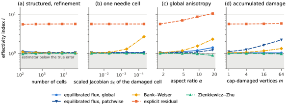
Figure 2: Effectivity indices, test case (T1), for the two reconstructions of the guaranteed bound and the three competitors. (a) uniform refinement of the structured mesh; (b) a single needle cell whose scaled Jacobian is swept over four decades, the rest of the mesh being untouched; (c) increasing global anisotropy; (d) an increasing number $m$ of cap-damaged vertices grouped in a contiguous block, at fixed local quality $s_{K} = 1 0^{- 3} .$ In the shaded band the estimator is below the true error: neither reconstruction of the guaranteed bound ever enters it, the Zienkiewicz–Zhu estimator never leaves it. Panel (b) is the sharpest contrast of the campaign: one degenerate cell out of $2048$ leaves the equilibrated index at $1.032$ and multiplies the Bank–Weiser index by $2. 6 .$ Panels (c) and (d) are mirror images of one another: anisotropy degrades the global reconstruction and leaves the patchwise one flat, accumulated damage does the reverse (Section 10.8).

10.5 Randomly perturbed meshes

The first three rows of Table 3 perturb every interior vertex. As $δ$ grows from $0.10$ to $0.3 0,$ the worst scaled Jacobian falls from $0.56$ to $0.23$ and the largest angle climbs from $107$ to $147$ degrees, i.e. the mesh becomes one that most quality-control tools would reject. The equilibrated effectivity index moves from $1.033$ to $1.03 4 :$ it is, for practical purposes, constant. The recovery estimator, on the other hand, drifts from $0.989$ to $0.96 1 :$ the perturbation destroys the superconvergence on which its accuracy rests, and it does so in the unsafe direction. Bank–Weiser degrades mildly and safely, $1.022$ to $1.06 2,$ losing its advantage over the equilibrated flux by $δ = 0.30$ without ever falling below one.

10.6 Locally damaged meshes, and the extent of the damage

The next eight rows of Table 3 displace a single vertex. Between $t = 10^{- 1}$ and $t = 10^{- 4}$ the scaled Jacobian of the damaged cell drops by three orders of magnitude, down to $s_{K} = 5 \cdot 10^{- 5}$ for the needle and $10^{- 4}$ for the cap, and $θ_{\max}$ reaches $180.0$ degrees to the printed precision. The response of the estimator is nil: $I^{e q} = 1.032$ throughout, to four digits, and the cellwise sharpness on the damaged cell itself, $I_{K}^{b a d},$ stays at $1.0 0 .$ An isolated degenerate cell — of either type, needle or cap — is simply invisible to the equilibrated flux estimator. This is the numerical counterpart of Theorem 7.9: nothing in its proof could have noticed. It is not invisible to Bank–Weiser, whose index reaches $2.664$ on the thinnest needle; we come back to this in Section 10.10, since it is the clearest difference the two local-problem estimators exhibit.

Table 4 isolates the effect of the extent of the damaged region, family (F4): the number $m$ of degenerate cells and their local quality are held fixed, only their spatial arrangement changes.


mesh	$m$	$diam / h$	$I^{e q}$	$I^{B W}$	$I_{K}^{b a d}$
F4 scattered $m = 1$	1	0.0	1.0323	1.019	1.00
F4 block $m = 1$	1	0.0	1.0321	1.028	1.00
F4 scattered $m = 4$	4	27.9	1.0321	1.032	1.06
F4 block $m = 4$	4	2.8	1.0314	1.058	1.00
F4 scattered $m = 16$	16	34.4	1.0311	1.095	1.06
F4 block $m = 16$	16	8.9	1.0297	1.152	1.00
F4 scattered $m = 64$	64	36.9	1.0307	1.198	1.14
F4 block $m = 64$	64	19.8	1.0278	1.321	1.02

Table 4: Family (F4): $m$ cap-damaged vertices at fixed $t = 10^{- 3}$ (hence fixed $s_{K} = 10^{- 3}$ and $θ_{\max} = 179.9$ degrees), test case (T1), $N = 3 2 .$ Only the diameter of the damaged region changes between the scattered and the block rows at equal $m .$ Note that $I^{B W}$ responds to the accumulation of damage where $I^{e q}$ does not.

Two conclusions, one of which is negative and worth stating as such.

The global index is remarkably stable, $1.0278 \leq I^{e q} \leq 1.032 3,$ and if anything decreases as damage accumulates: a damaged mesh is a slightly finer mesh, and the estimator tracks the error it actually commits.
With the global reconstruction, the experiment does not discriminate the conjecture of Section 7.3. At equal $m,$ the contiguous block (diameter $19.8 h$ at $m = 6 4)$ behaves marginally better than the scattered layout (diameter $36.9 h),$ $I_{K}^{b a d} = 1.02$ against $1.1 4,$ and the differences are within the variation caused by where in $Ω$ the damaged cells happen to fall, since $| | | u - u_{h} | | |_{K}$ itself varies by an order of magnitude across the domain. This is a limitation of the reconstruction, not of the mesh family: the conjecture is about the local efficiency constant $C_{s t} (γ_{ω_{K}}),$ and the global reconstruction exposes no local constant. Section 10.8 redoes the experiment with the patchwise reconstruction, which does, and settles the question — against the conjecture as we stated it.

10.7 Anisotropic meshes

The last four rows of Table 3 are the only ones on which the equilibrated estimator visibly degrades: $I^{e q}$ grows from $1.032$ to $1.401$ as the cells are stretched from aspect ratio $1$ to about $1 6,$ and the cellwise sharpness on the worst cells reaches $I_{K}^{b a d} = 1.8 7 .$ This is consistent with Theorem 7.14 and with the distinction we have insisted on: anisotropy is a global loss of shape regularity — every cell is bad — whereas the damage of family (F3) is local. The guarantee is of course untouched; what is lost is sharpness, and it is lost gradually. For comparison, $I^{r e s}$ nearly doubles over the same range, from $5.63$ to $10.4 3,$ which is the practical statement that no fixed calibration constant $C$ can serve both a structured and an anisotropic mesh. Bank–Weiser degrades faster than either, $1.017$ to $2.29 7,$ crossing the equilibrated flux between $α = 1$ and $α = 4 .$

10.8 The two reconstructions of the same bound

Everything reported so far uses the global mixed reconstruction of Section 7.4. Table 5 adds the patchwise one of Section 7.5, at the degree $p = k = 1$ prescribed by [EV15] and at the cheapest admissible degree $p = 0 .$ The two reconstructions certify the same quantity with the same constant; they differ only in sharpness, and the comparison is instructive because they do not lose sharpness under the same defects.


mesh	$I^{e q}$	$I^{p w}$ $(p = 1)$	$I^{p w}$ $(p = 0)$	$I^{B W}$
F1 $N = 8$	1.130	1.053	1.295	1.082
F1 $N = 16$	1.065	1.049	1.240	1.037
F1 $N = 32$	1.032	1.048	1.226	1.017
F1 $N = 64$	1.016	1.047	1.247	1.008
F1 $N = 128$	1.008	1.047	1.309	1.004
F2 $δ = 0.30$	1.034	1.055	1.790	1.062
F3 needle $t = 10^{- 4}$	1.032	1.048	1.226	2.664
F3 cap $t = 10^{- 4}$	1.032	1.112	1.238	1.028
F4 scattered $m = 64$	1.031	1.812	3.373	1.198
F4 block $m = 64$	1.028	2.215	2.864	1.321
F5 $32 \times 32$	1.032	1.048	1.226	1.017
F5 $32 \times 8$	1.092	1.036	1.253	1.163
F5 $32 \times 4$	1.182	1.070	1.357	1.529
F5 $32 \times 2$	1.401	1.220	1.638	2.297

Table 5: Effectivity indices of the two reconstructions of the guaranteed bound, test case (T1). $I^{e q}$ is the global mixed reconstruction of Section 7.4, $I^{p w}$ the patchwise one of Section 7.5. The global one degrades under global anisotropy and ignores local damage; the patchwise one does the opposite. The $p = 0$ column shows that the degree of the local space is not a free parameter.

Three observations.

The degree $p$ is not free. At $p = 1$ the patchwise index is flat at $1.04 7 –$ $1.053$ over the whole structured family. At $p = 0$ it is not merely larger $(1 .23$ to $1.3 1)$ but non-monotone under refinement, so that the reconstruction no longer converges at the rate of the error. The bound of Theorem 7.9 holds for either — any admissible $σ_{h}$ gives a valid certificate — but only $p = k$ delivers a sharp one. This is the numerical face of the $p -$ robustness theory of [BPS09, EV20], and it is worth stating explicitly, since $p = 0$ is the natural choice for a practitioner who reads only the reliability statement.
Anisotropy costs the global reconstruction, not the patchwise one. Over the family (F5), $I^{e q}$ grows from $1.032$ to $1.401$ while $I^{p w}$ stays between $1.036$ and $1.22 0;$ at aspect ratio $4$ the patchwise index is actually smaller than on the isotropic mesh. The same holds on the under-resolved boundary layer, where $I^{p w} = 1.583$ against $I^{e q} = 2.402$ (Table 7).
Accumulated damage costs the patchwise reconstruction, not the global one. The two indices exchange roles on family (F4): at $m = 64$ cap-damaged vertices in a contiguous block, $I^{e q} = 1.028$ while $I^{p w} = 2.21 5 .$ Notably, a needle leaves the patchwise index untouched $(1 .04 8)$ while a cap of the same scaled Jacobian moves it to $1.112$ — the reverse of the Bank–Weiser behaviour of Section 10.10, which is blind to caps and sensitive to needles.

Panels (c) and (d) of Figure 2 display the exchange directly: the two curves cross over from one panel to the other, while the three competitors behave the same way in both.

The practical reading is that the guarantee is a property of the framework and the sharpness a property of the reconstruction, and that no single reconstruction is uniformly sharpest. Since both certificates are valid, the sharper of the two may simply be retained: the minimum of two guaranteed bounds is a guaranteed bound. Over the whole campaign that minimum never exceeds $1.22$ on the smooth test case.

The damage-extent conjecture.

Section 10.6 could not discriminate the conjecture of Section 7.3 because the global reconstruction exposes no local efficiency constant. The patchwise one does, and it answers the question — in the negative, as stated. At equal $m$ and equal local quality, the block layout is systematically worse than the scattered one: $1.239$ against $1.123$ at $m = 4,$ $1.624$ against $1.407$ at $m = 1 6,$ $2.215$ against $1.812$ at $m = 6 4 .$ Yet the block has the smaller diameter $(1 9.8 h$ against $36.9 h$ at $m = 6 4,$ Table 4). The diameter of the damaged region is therefore not the relevant parameter; what degrades $C_{s t}$ is the number of flattened cells sharing a single vertex patch, which is exactly the quantity that enters the local efficiency proof and which the block layout maximises at fixed $m .$ We record this as the corrected form of the conjecture.

10.9 Does any quality measure predict the effectivity?

Section 6 introduced the quality vector $q_{K}$ of (10) and announced that it would be correlated with the local effectivity index. Table 6 reports the empirical Pearson correlation $ρ (I_{K}, \cdot)$ between each component and the local index $I_{K}$ of (11), computed with the patchwise reconstruction — the denominator being the patch error, which is what Theorem 7.14 actually bounds.


mesh	$ρ (I_{K}, γ_{K})$	$ρ (I_{K}, α_{K})$	$ρ (I_{K}, s_{K})$	$ρ (I_{K}, κ_{K})$	$ρ (I_{K}, θ_{\min})$	$ρ (I_{K}, θ_{\max})$
F2 $δ = 0.10$	-0.03	-0.04	0.08	-0.04	0.08	-0.01
F2 $δ = 0.20$	-0.07	-0.08	0.11	-0.09	0.10	-0.02
F2 $δ = 0.30$	-0.11	-0.13	0.14	-0.14	0.12	-0.03
F3 needle $t = 10^{- 4}$	-0.25	-0.25	0.16	-0.25	0.15	-0.04
F3 cap $t = 10^{- 4}$	0.01	0.01	-0.32	0.01	-0.33	0.27
F4 scattered $m = 64$	0.12	0.12	-0.36	0.12	-0.36	0.30
F4 block $m = 64$	0.19	0.19	-0.48	0.19	-0.47	0.33

Table 6: Correlation between the local effectivity index (11) and each component of the quality vector (10), test case (T1), $N = 3 2 .$ No component reaches $| ρ | = 0. 5,$ and the sign of $ρ (I_{K}, γ_{K})$ flips between the needle and the cap families.

The outcome is a negative result, and we regard it as the useful one.

No measure predicts the effectivity. The largest correlation over the whole table is $| ρ | = 0.4 8,$ for $s_{K}$ on the block-damaged mesh. A quality report is not a proxy for an error bound, which is the practical form of the message of Table 1.
The sign is not even stable. $ρ (I_{K}, γ_{K})$ is $- 0.25$ on the needle family and $+ 0.19$ on the block-damaged one. A shape-regularity ratio that grows can accompany either an increase or a decrease of the local effectivity, depending on how the cell degenerates. This is Babuška and Aziz [BA76] seen from the a posteriori side.
Three of the six measures carry the same information. The columns $γ_{K},$ $α_{K}$ and $κ_{K}$ agree to two decimals on the damaged families, and to within $0.03$ on the perturbed ones. Two reasons combine: for a triangle $κ_{K} = (α_{K} + α_{K}^{- 1}) / 2$ is an exact function of $α_{K};$ and on a mesh in which all cells but a few carry the same quality value, the correlation coefficient is determined by which cells are outliers and not by how large the outlying values are. The measures that do separate the families are $s_{K}$ and the extremal angles.

10.10 Bank–Weiser: sharper on good meshes, more fragile on bad ones

The $I^{B W}$ column of Tables 2–7 deserves to be read on its own, because it is the only competitor that is a serious one.

On good meshes it wins.

On the structured family, $I^{B W}$ falls from $1.082$ to $1.004$ while $I^{e q}$ falls from $1.130$ to $1.00 8 :$ Bank–Weiser overestimates by about half as much, at every refinement level, and both are asymptotically exact. On the under-resolved boundary layer (T3) the gap is wider still, $1.743$ against $2.40 2 .$ If sharpness on a reasonable mesh were the only criterion, Bank–Weiser would be the estimator to use — which is presumably why it is.

A single needle cell costs it a factor of $2. 6 .$

The needle rows of Table 3 are the sharpest contrast of the whole campaign. As $t$ goes from $10^{- 1}$ to $1 0^{- 4},$ $I^{e q}$ stays at $1.032$ to four digits, while $I^{B W}$ climbs $1.021 \to 1.048 \to 1.282 \to 2.66 4 .$ One cell out of $204 8,$ and the Bank–Weiser estimator has lost a factor of $2. 6;$ the equilibrated one has not moved. Figure 2(b) plots exactly this.

The cap rows show nothing of the sort: $I^{B W}$ moves from $1.023$ to $1.028$ and then stops. The two damages have comparable scaled Jacobians (within a factor of two at equal $t)$ and the same shape-regularity ratio $γ_{K} \approx 200 0,$ so $γ_{K}$ does not explain the difference. What distinguishes them is that the needle collapses an edge — two vertices come to within $t h$ of each other — whereas the cap collapses only the area, all three edges keeping length $O (h) .$ The Bank–Weiser space (35) is spanned by the edge bubbles, so an edge of length $t h$ carries a basis function whose gradient blows up like $(t h)^{- 1},$ and the local problem (36) is solved in a space that is badly scaled against the residual it must represent. We offer this as the plausible mechanism rather than as a proof; what the experiment establishes is the fact, and the fact is that the relevant geometric parameter for Bank–Weiser is not the one the quality-control tool reports.

Anisotropy and accumulated damage cost it too.

Over the anisotropic family, $I^{B W}$ grows from $1.017$ to $2.297$ against $1.032$ to $1.401$ for the equilibrated flux: the two estimators start with Bank–Weiser ahead and end with it $60 %$ behind (Figure 2(c)). The same crossing happens as damage accumulates in family (F4), Table 4: at $m = 64$ in a contiguous block, $I^{B W} = 1.321$ against $I^{e q} = 1.02 8 .$

The diffusion contrast breaks the unweighted variant.

The largest entry of the campaign is the last row of Table 7: with $μ$ jumping by $10^{4}$ across a mesh-aligned interface, $I^{B W} = 12.514$ where $I^{e q} = 1.03 2 .$ This is remark (c) of Section 8 made quantitative. The facet term of (36) carries $μ = 10^{4}$ from the high-coefficient side, and on the low-coefficient cell it is weighed against $μ = 1$ in the local bilinear form; the estimator therefore attributes to that cell an error four orders of magnitude too large.

Coefficient-weighted averages are the known cure, and we have measured them, so as not to charge the estimator with a defect of one particular variant. Replacing the $1 / 2$ split of (36) by the weights $ω_{K} = μ_{K} / (μ_{+} + μ_{-})$ — which give the low-coefficient side a share of the jump proportional to its own $μ,$ and restore the $μ_{\max}^{- 1 / 2}$ scaling of the residual estimator (33) — brings the index from $12.514$ down to $1.01 4,$ and changes nothing at all on the runs with constant $μ,$ where the two variants agree to machine precision. The column $I^{{B W}_{μ}}$ of Table 7 reports it. The $12.5$ is therefore entirely an artefact of the unweighted split, and the statement that survives is the one about who has to know: the contrast-robustness of the equilibrated flux estimator is a theorem [CZ12] that requires nothing of the user, whereas that of Bank–Weiser is a modelling choice that has to be got right, silently, before the computation.

It does underestimate, and nothing signals it.

Across the $32$ synthetic runs on the unit square and the one real mesh with a known solution, $I^{B W}$ stayed above one, with a minimum of $1.00 4;$ Bank–Weiser should therefore not be lumped together with Zienkiewicz–Zhu, which was below one every single time. On the L-shaped domain, however, it is below one on all four meshes, down to $I^{B W} = 0.9935$ (Table 8). The deficit is small, under a percent, and a practitioner would not notice it. The saturation assumption on which reliability rests is not satisfied there, nothing in the computed output says so, and the estimator returns a number that is confidently below the truth. The difference with the equilibrated flux is not that the latter is sharper, but that its failure mode is a certificate one can check (step 4 of Algorithm 7.19) rather than an assumption one must believe.

Cost.

On the finest structured mesh $(3 2 768$ cells), the primal solve takes $0.13$ s, the Bank–Weiser estimator $0.27$ s and the global mixed reconstruction $1.10$ s: Bank–Weiser costs about twice the primal solve, the global equilibrated reconstruction about eight times. We deliberately do not quote a wall-clock figure for the patchwise reconstruction. Its $16 641$ local systems have at most $43$ unknowns each, so its arithmetic content is well below one second of dense linear algebra; but our driver loops over the patches in Python and spends $5.5$ s doing so, which measures the interpreter and not the method. The meaningful statement is the algebraic one: per vertex, one dense symmetric system of size at most $4 3,$ all of them independent, against one global saddle-point solve for the reconstruction of Section 7.4 and one $3 \times 3$ system per cell for Bank–Weiser.

10.11 Boundary layers and heterogeneous coefficients

Table 7 collects the other two test cases on the structured $32 \times 32$ mesh.


case		$\| \| \| u - u_{h} \| \| \|$	$I^{e q}$	$I^{p w}$	$I^{B W}$	$I^{{B W}_{μ}}$	$I^{Z Z}$
(T1)	smooth, $μ = 1$	1.090e-01	1.032	1.048	1.017	1.017	0.993
(T3)	layer, $ε = 10^{- 2}$	1.178e+00	2.402	1.583	1.743	1.743	0.414
(T4)	$μ$ contrast $10^{4}$	7.705e+00	1.032	1.048	12.514	1.014	0.993

Table 7: Test cases (T1), (T3), (T4) on the structured mesh (F1) with $N = 3 2,$ $k = 1 .$

Boundary layer.

With $ε = 10^{- 2}$ and $h = 1 / 3 2,$ the layers are heavily under-resolved and the discrete solution carries an error of the order of the solution itself. The equilibrated estimator reports it: $I^{e q} = 2.4 0,$ i.e. it announces an error at most $2.4$ times the true one — pessimistic, but the announcement is of the right order and it is a guarantee. The recovery estimator announces $I^{Z Z} = 0.4 1,$ i.e. it reports two and a half times less error than there is. On a pre-asymptotic mesh, where the user most needs to be warned, the popular estimator is the one that gives false confidence. This is, in our view, the most consequential single figure of the campaign. Bank–Weiser, for its part, is the sharpest of the four here, $I^{B W} = 1.7 4,$ and stays above one — on this test case the saturation assumption evidently holds.

Heterogeneous coefficient.

With a contrast of $10^{4}$ across a mesh-aligned interface, the effectivity indices of the equilibrated flux, of the recovery and of the residual estimator are unchanged from the homogeneous case $(1 .032$ against $1.03 2,$ $0.993$ against $0.99 3,$ and $5.632$ against $5.64 3)$ — but not that of Bank–Weiser, which jumps from $1.017$ to $12.51 4;$ its coefficient-weighted variant returns $1.01 4 .$ See Section 10.10. This confirms numerically the $μ -$ robustness of Theorem 7.9: the coefficient enters only through the weights $μ^{\pm 1 / 2},$ and no constant sees the contrast. The patchwise reconstruction behaves identically, $I^{p w} = 1.048$ against $1.04 8 .$

Assumption (M3) is not decorative either, but its failure is not one that the certificate can see. Repeating the run with the damaged vertex placed on the interface, so that it is dragged across it and $μ$ ceases to be constant on the three cells it drags along (interface_check.py in the repository), the equilibration defect stays at $3.7 \cdot 1 0^{- 11} :$ the mixed problem (26) equilibrates $σ_{h}$ against whatever $f$ it is given, and (EF) holds whatever $μ$ does inside a cell. What (M3) controls is the residual indicator. Its proof inserts $μ_{K}^{- 1 / 2},$ which on a crossed cell has to be replaced by $(\min_{K} μ)^{- 1 / 2}$ — the bound survives — and, more importantly, $f - Π_{0} f$ is no longer of higher order there, since $f$ jumps by a factor $10^{4}$ inside the cell. The discrete solution itself is barely affected, $| | | u - u_{h} | | | = 7.73$ against $7.7 1,$ but the ratio $‖ η^{R} ‖ / ‖ η^{F} ‖$ rises from $0.04$ to above $1,$ reaching $4.4$ on the crossed cells, and the guaranteed index becomes $I^{e q} = 9. 2 .$ The bound is still a bound, and it still holds by virtue of Theorem 7.9 once the weight is corrected, but it has lost its sharpness because of three cells out of $204 8;$ the signal is in the oscillation column of the output, not in the certificate. Whether $μ$ is constant on every cell is, in any case, a property of the data that can be checked by inspection before the computation, which is why we do not count (M3) among the hypotheses the certificate is responsible for.

10.12 The L-shaped domain: dropping a hypothesis on purpose

Remark 7.11 identifies the one hypothesis of Theorem 7.9 that we cannot enforce in practice: that the discrete boundary values coincide with $g .$ Test case (T2) on the meshes (F7) violates it — $g_{h}$ is the Lagrange interpolant of $r^{2 / 3} \sin (2 θ / 3),$ so $u - u_{h} / \in H_{0}^{1} (Ω)$ and the theorem does not apply. Table 8 reports what happens.


mesh	cells	$\| \| \| u - u_{h} \| \| \|$	rate	$I^{e q}$	$I^{p w}$	$I^{B W}$	$I^{Z Z}$
F7 L-shape $N = 4$	96	1.898e-01	—	1.110	1.187	0.9992	1.062
F7 L-shape $N = 8$	384	1.221e-01	0.64	1.105	1.177	0.9951	1.056
F7 L-shape $N = 16$	1536	7.799e-02	0.65	1.103	1.172	0.9939	1.053
F7 L-shape $N = 32$	6144	4.957e-02	0.65	1.101	1.169	0.9935	1.052

Table 8: Test case (T2) on the L-shaped meshes (F7), $k = 1 .$ The observed convergence rate $0.65$ matches the expected $h^{2 / 3} .$ Theorem 7.9 does not cover these runs, the Dirichlet datum being interpolated rather than exact; both reconstructions nevertheless stay above the true error, whereas Bank–Weiser is below it on every mesh of the family.

Three observations, the first two of which qualify the guarantee rather than support it.

The bound survives, but we cannot claim it. Both $I^{e q} = 1.10 1 –$ $1.110$ and $I^{p w} = 1.16 9 –$ $1.187$ stay comfortably above one, and remarkably stable across four refinements of a singular solution. This is evidence that the boundary term neglected here is small on this family, not that it is small in general; on a coarser mesh or with a rougher datum it need not be. We report the numbers as an indication, and repeat that the certificate of step 4 of Algorithm 7.19 does not detect this failure — it tests (EF), which still holds exactly here (the defect is at $1 0^{- 13}),$ and is silent about the boundary condition. This is the one gap in the guarantee that the computation cannot check.
Bank–Weiser underestimates. $I^{B W}$ is $0.999 2,$ $0.995 1,$ $0.993 9,$ $0.9935$ on the four meshes: below one every time, and drifting further below under refinement. This is the only family of the campaign on which it does so, and it is a shape-regular one — the difficulty is the corner singularity, not the geometry of the cells. It confirms, on a textbook test case, that the empirical safety observed in Section 10.10 is a property of the problems tested and not of the estimator.
Zienkiewicz–Zhu is above one here. $I^{Z Z} = 1.0 5,$ the only place in the campaign where it does not underestimate. Recovery estimators are not systematically unsafe; they are unsafe where superconvergence holds and their calibration is tuned to it, which is the smooth, structured regime. On a singular solution the recovered gradient is simply too rough, and the estimator errs the other way. Neither behaviour is under control.

10.13 A certified quantity of interest

Table 9 applies Proposition 9.1 to the mean of $u$ over the box $D = (1 / 4, 1 / 2)^{2},$ on test case (T1) where $J (u)$ is known in closed form. The dual problem $- div (μ \nabla z) = | D |^{- 1} 1_{D}$ is solved with the same factorised matrix as the primal one, and the same reconstruction is applied to it.


mesh	cells	$\| J (u) - J (u_{h}) \|$	$η^{p r i m}$	$η^{d u a l}$	bound	$I^{g o a l}$
F1 $N = 8$	128	2.839e-02	4.878e-01	1.536e-01	7.493e-02	2.64
F1 $N = 16$	512	7.167e-03	2.316e-01	7.974e-02	1.847e-02	2.58
F1 $N = 32$	2048	1.796e-03	1.125e-01	4.036e-02	4.541e-03	2.53
F1 $N = 64$	8192	4.493e-04	5.540e-02	2.026e-02	1.122e-03	2.50
F2 $δ = 0.30$	2048	2.083e-03	1.208e-01	4.951e-02	5.981e-03	2.87
F3 needle $t = 10^{- 4}$	2048	1.788e-03	1.128e-01	4.149e-02	4.680e-03	2.62
F3 cap $t = 10^{- 4}$	2048	1.808e-03	1.130e-01	4.109e-02	4.642e-03	2.57
F5 $32 \times 2$	128	2.037e-01	1.633e+00	5.842e-01	9.539e-01	4.68

Table 9: Guaranteed bound (38) on the quantity of interest $J (v) = | D |^{- 1} \int_{D} v,$ $D = (1 / 4, 1 / 2)^{2},$ test case (T1). The goal error converges at $h^{2}$ and so does the product bound, so the effectivity index is asymptotically constant. As for the energy bound, an isolated degenerate cell leaves it essentially unchanged and global anisotropy degrades it.

The bound held in all eight runs. The effectivity index sits at $2.5 0 –$ $2.64$ on the structured family and decreases monotonically under refinement, which is the expected behaviour: $| J (u) - J (u_{h}) |$ and the product $η^{p r i m} η^{d u a l}$ both converge at $h^{2},$ and what the index measures is the cancellation between the primal and the dual error distributions that the Cauchy–Schwarz step of (38) throws away. A factor of $2.5$ is the price of a product bound; it is not the price of the mesh. The mesh enters exactly as it does in the energy norm: a needle or a cap with $s_{K} = 10^{- 4}$ moves the index from $2.53$ to $2.62$ and $2.57$ respectively, while the aspect-ratio- $16$ mesh takes it to $4.68$ — the compounding of the degradation seen on each factor separately, which is what a product of two bounds must do. A quantity of interest computed on a mesh containing a degenerate cell can therefore be certified at essentially the same price, and with the same constant, as the energy norm.

10.14 Summary of the campaign

The campaign comprises $49$ computations: $32$ runs on the unit square covered by Theorem 7.9, $4$ runs on the L-shaped domain that are not (Section 10.12), $8$ goal-oriented runs (Section 10.13) and the $5$ real meshes of Section 10.15. Over the runs covered by the theorem:

the guaranteed bound $η \geq | | | u - u_{h} | | |$ held in every run where the error is computable, the assertion of Listing 1 never firing, for either reconstruction, and the goal-oriented bound (38) held in all $8$ of its runs;
$I^{e q} \in [1.008, 2.402],$ the upper end being reached only on the deliberately under-resolved boundary layer; on the smooth test case it never exceeded $1.40 1,$ whatever the distortion;
$I^{p w} \in [1.036, 2.215]$ for the patchwise reconstruction at $p = k,$ the upper end being reached on accumulated cap damage rather than on anisotropy: the two reconstructions of the same bound fail to be sharp on disjoint families of meshes (Section 10.8);
$I^{Z Z} < 1$ in all $32$ synthetic runs, with a worst case of $0.41 4;$
$I^{B W} \in [1.004, 12.514] :$ the sharpest estimator on good meshes and the most fragile on bad ones. It stayed above one on the unit square, but fell to $0.9935$ on the L-shaped domain; its coefficient-weighted variant removes the $12.514$ — it ranges over $[1.004, 2.664]$ — but not the underestimation;
$I^{r e s}$ ranged over $[5.53, 10.43],$ a factor of almost two between the extreme meshes, so that no universal calibration of $C$ exists;
the relative equilibration defect never exceeded $7.2 \cdot 10^{- 10}$ for the global reconstruction and $4.4 \cdot 10^{- 10}$ for the patchwise one, boundary layer included.

Two hypotheses were violated on purpose, and the outcome sorts the hypotheses of Theorem 7.9 into three classes. Assumption (M3) — a coefficient interface crossing a cell — is a property of the data, checkable by inspection before any computation; its violation leaves the bound valid but raises the effectivity index from $1.03$ to $9. 2,$ and the certificate does not see it. The equilibration (EF) is a property of the reconstruction, and the certificate of step 4 of Algorithm 7.19 checks it (the $H (div) -$ conformity of $σ_{h}$ holds by construction of the space). The exactness of the discrete Dirichlet datum (Remark 7.11) is checkable by neither, and this is worth stating plainly: it is the one hypothesis for which the computed output cannot vouch.

10.15 Real geometries

We close with the meshes that reached us from the applications this work originates in, family (F6). They come as OFF files and illustrate the two situations of engineering practice.

A mesh that no solver will accept.

The file square_good.1.off triangulates $(- 1, 1)^{2}$ with $801$ right triangles. Its quality figures are those of a perfectly structured mesh, $s_{K} \equiv 0.707$ and $θ_{\max} = 90$ degrees — and it contains one cell of exactly zero area, because two of its vertices are the same point to machine precision. This is not an exotic pathology: the file is named “good”, nothing in its quality report signals the defect, and every finite element code will produce a singular system from it. Our reader (offio.py) reports the defect, merges the coincident vertices and drops the degenerate cell, leaving $800$ cells. Since the domain is then exactly the square, the manufactured solution $u = \cos (π x_{1} / 2) \cos (π x_{2} / 2)$ applies and the effectivity index can be measured: $I^{e q} = 1.054$ (Table 10). The guarantee holds on a mesh that was not prepared for the experiment.

A mesh whose exact solution nobody knows.

The four remaining meshes triangulate the letter “A” — a non-convex domain with thin features, sharp corners and re-entrant corners — and come from two different meshers (as, unstructured and graded; aa, uniform) at two refinement levels each. No closed-form solution is available, which is the normal state of affairs. We solve $- Δ u = 1$ with homogeneous Dirichlet data and report the certified quantity that a practitioner would actually obtain: the bound $η,$ and its size relative to the energy of the computed solution.


mesh	cells	$s_{\min}$	$θ_{\max}$	$η$	$η / \| \| \| u_{h} \| \| \|$	$I^{e q}$	$η^{B W} / η$	$η^{p w} / η$	defect
as6	1327	0.23	143.4	1.551e-03	28.1%	—	1.103	1.065	$1 \cdot 10^{- 14}$
as7	3262	0.26	145.3	1.166e-03	20.8%	—	1.130	1.054	$3 \cdot 10^{- 14}$
aa6	1983	0.25	143.4	1.111e-03	19.8%	—	1.035	1.062	$7 \cdot 10^{- 14}$
aa7	7924	0.26	145.3	5.979e-04	10.5%	—	0.986	1.067	$3 \cdot 10^{- 13}$
square_good	800	0.71	90.0	1.797e-01	8.1%	1.054	1.047	0.997	$7 \cdot 10^{- 14}$

Table 10: Family (F6), the real meshes. The four glyph meshes solve $- Δ u = 1$ and no exact solution is available, so only the certified bound is reported; square_good carries a manufactured solution and its effectivity index is measured. The penultimate column compares the Bank–Weiser bound to the guaranteed one: on these meshes the two agree within $13 % .$ The next column does the same for the patchwise reconstruction, which agrees with the global one within $7 %$ on all five meshes. The last column is the relative equilibration defect of step 4 of Algorithm 7.19.

Three things come out of Table 10 and Figure 3.

The bound is informative, not vacuous. On aa7 the energy-norm error is certified to be at most $10.5 %$ of the energy of the computed solution; on as6 at most $28.1 % .$ These are numbers an engineer can act on, obtained without knowing $u .$
It ranks the meshers. At $1983$ cells, aa6 certifies $19.8 %,$ whereas as7 needs $3262$ cells — $64 %$ more — to certify a slightly worse $20.8 % .$ For this problem the uniform mesher is the more efficient of the two, and the guaranteed bound says so without any reference computation. Comparing two meshers objectively on a geometry where the solution is unknown is, to our knowledge, not otherwise possible without a reference computation.
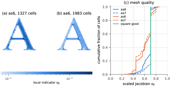
It localises the error where one expects it. Figure 3(a,b) maps $η_{K} :$ the indicator concentrates in the crossbar of the glyph, where the cells are elongated and where the two re-entrant corners sit. Panel (c) confirms that the two meshers differ in quality — the aa family is uniformly better in scaled Jacobian — but that both stay in the comfortable range $s_{K} \geq 0.2 3 :$ these real meshes are far less distorted than the synthetic ones of Table 3, so that what they test is the geometry of the domain rather than the geometry of the cells.

Figure 3: The real meshes of family (F6). (a), (b) the local indicator $η_{K}$ on the two coarse glyph meshes, on a common logarithmic colour scale; the error concentrates in the crossbar and at the re-entrant corners. (c) cumulative distribution of the scaled Jacobian: hue distinguishes the mesher, dashing the refinement level.

The patchwise reconstruction behaves on these meshes as it does on the synthetic ones, returning a bound within $7 %$ of the global one (Table 10) — unsurprisingly, since by Figure 3(c) these meshes contain no flattened cell of the kind that Section 10.8 identified as its weak point. A quantity of interest on this geometry — say the mean of $u$ over the crossbar — would be certified by (38) at the price of one extra solve, exactly as in Section 10.13; we have not run it, since no reference value of $J (u)$ exists here against which the resulting bound could be calibrated.

11 Conclusion and perspectives

We have argued, and demonstrated on $49$ numerical experiments, that equilibrated flux estimators answer a question that practitioners actually ask — how wrong is my computation on this mesh? — in a regime where the standard tools are silent: coarse meshes, distorted cells, no asymptotics. The guarantee comes with a constant equal to one and, remarkably, with no geometric assumption; the price is a possible loss of sharpness, which is the benign failure mode.

The campaign of Section 10 supports this rather sharply. An isolated degenerate cell, needle or cap, with a scaled Jacobian of $5 \cdot 10^{- 5}$ and a maximum angle of $180$ degrees to printed precision, changes the effectivity index of the equilibrated estimator by less than $1 0^{- 3};$ global anisotropy degrades it, but only from $1.03$ to $1.4 0;$ and it never fell below one. Over the same runs the Zienkiewicz–Zhu estimator was below one every single time, reaching $0.41$ on an under-resolved boundary layer — reporting less than half of the error actually committed, in the very situation where a warning is needed.

The comparison with Bank–Weiser is the most informative one, that estimator being both accurate and widely used, so that the trade-off is visible in the numbers. It is sharper than the equilibrated flux on every well-shaped mesh, by roughly a factor of two in the overestimation, and sharper still on the under-resolved layer. It is also the estimator that distortion punishes most: a single needle cell out of $2048$ multiplies its index by $2. 6,$ global anisotropy by $2. 3,$ a coefficient contrast of $10^{4}$ by $12$ — each time while the guaranteed index stays at $1.0 3 .$ Of these, the last is removable: a coefficient-weighted facet split brings the $12$ back to $1.01$ (Section 10.10). The first two are not, and the L-shaped domain adds a failure that no calibration repairs, the estimator falling below the true error on every mesh of that family while returning no indication that it has. Sharpness and robustness are traded against each other here, and which one a practitioner should buy depends on whether the mesh is one they chose.

Two findings were not anticipated when the campaign was designed, and they are the ones we would single out. First, the two reconstructions of the same guaranteed bound — the global mixed one and the patchwise one — lose sharpness on disjoint families of meshes: the global one under global anisotropy, the patchwise one under an accumulation of flattened cells inside a single vertex patch. Since both are certificates, the sharper of the two may simply be kept, and their minimum is again guaranteed. Second, no component of the quality vector (10) predicts the local effectivity index: the largest correlation over the campaign is $0.4 8,$ and the sign of the correlation with the shape-regularity ratio reverses between a needle and a cap (Section 10.9). A mesh-quality report and an error bound answer different questions, and the second cannot be inferred from the first.

Open directions:

Sharp characterisation of admissible distortion. Following [DLL19], find a necessary and sufficient condition on the damaged region for the effectivity index to stay bounded. Section 10.8 rules out the diameter of the damaged region as the relevant parameter and points instead to the number of flattened cells sharing a vertex patch; turning that observation into a bound on $C_{s t}$ is open.
Three dimensions. Theorem 7.9 is written for $d \in {2, 3}$ and the Payne–Weinberger constant does not depend on the dimension, so the guarantee transfers verbatim to tetrahedral meshes. The sharpness does not: in the experience of one of us with three-dimensional eddy-current problems, the lowest-order reconstruction in ${R T}_{0}$ leaves the effectivity index well above one, and the ${R T}_{1}$ reconstruction that brings it back is expensive. Quantifying this trade-off on distorted tetrahedra — slivers, for which no two-dimensional analogue exists — is the natural continuation of the present campaign, and the anisotropic interpolation theory of [AADL11] suggests it is not hopeless.
Adaptivity on bad meshes. The convergence and optimality theory of AFEM [Dör96, CKNS08, NSV09] requires shape regularity; does Dörfler marking still behave well in practice when the initial mesh is distorted and cannot be improved?
Beyond Poisson. Elasticity (with the locking issue), Helmholtz [CFEV21], eddy currents and magnetodynamics [TLMC⁺13, CNT17]; also the linearisation and algebraic error components in the spirit of [EV13].
Extreme deformations. Estimators in the X-MESH setting [MRL⁺23], where elements are deliberately degenerated.
Meshless and immersed methods. Since no mesh enters the proof of Theorem 7.9, the framework should transfer.
Superconvergent postprocessing [MRV23] as a cheaper route to an equilibrated flux.
Non-homogeneous Dirichlet data. The one hypothesis of Theorem 7.9 that neither the data nor the certificate can vouch for (Remark 7.11). A computable bound on the boundary term, even a pessimistic one, would close the last gap between what is proved and what is run.

Code and data availability.

All the scripts, the input meshes and the raw result files needed to regenerate every table and every figure of this paper are openly available at

https://github.com/michelduprez/A-posteriori-error-estimation-for-coarse-or-distorted-meshes

The campaign runs in serial with FEniCSx (dolfinx 0.9.0); the repository README documents the role of each file and the exact commands used.

Acknowledgements.

This work was partially supported by the regional programme MATH-AmSud through the project NeuralFEM (2026–2027), which brings together teams from France, Uruguay, Chile and Colombia. This research is partly funded by la Fédération de Recherche d’Animation Bézout CNRS. We thank Roland Becker, Marek Bucki, Stéphane Bordas, Daniela Capatina, Alexei Lozinski, Robert Luce, Pascal Omnes, Yohan Payan, Martin Vohralik for highly stimulating discussions around this topic.

References

[AADL11] Gabriel Acosta, Thomas Apel, Ricardo G. Durán, and Ariel L. Lombardi. Error estimates for Raviart–Thomas interpolation of any order on anisotropic tetrahedra. Math. Comp., 80(273):141–163, 2011.

[AO00] Mark Ainsworth and J. Tinsley Oden. A Posteriori Error Estimation in Finite Element Analysis. Wiley, 2000.

[Ape99] Thomas Apel. Anisotropic finite elements: Local estimates and applications. Advances in Numerical Mathematics, 1999.

[BA76] Ivo Babuška and A. K. Aziz. On the angle condition in the finite element method. SIAM J. Numer. Anal., 13(2):214–226, 1976.

[BBF13] Daniele Boffi, Franco Brezzi, and Michel Fortin. Mixed Finite Element Methods and Applications, volume 44 of Springer Series in Computational Mathematics. Springer, 2013.

[BCL16] Roland Becker, Daniela Capatina, and Robert Luce. Local flux reconstructions for standard finite element methods on triangular meshes. SIAM J. Numer. Anal., 54(4):2684–2706, 2016.

[BDM85] Franco Brezzi, Jim Douglas, and L. Donatella Marini. Two families of mixed finite elements for second order elliptic problems. Numer. Math., 47(2):217–235, 1985.

$[BHL^{+} 23]$ Raphaël Bulle, Jack S. Hale, Alexei Lozinski, Stéphane P. A. Bordas, and Franz Chouly. Hierarchical a posteriori error estimation of Bank–Weiser type in the FEniCS Project. Comput. Math. Appl., 131:103–123, 2023.

[BK23] Sören Bartels and Alex Kaltenbach. Explicit and efficient error estimation for convex minimization problems. Math. Comp., 92(343):2247–2279, 2023.

[Ble16] Jan Blechta. dolfin-tape: DOLFIN tools for a posteriori error estimation. Software repository, 2016.

[BLP10] Marek Bucki, Claudio Lobos, and Yohan Payan. A fast and robust patient specific finite element mesh registration technique: Application to 60 clinical cases. Med. Image Anal., 14(3):303–317, 2010.

[BMV01] Christine Bernardi, Brigitte Métivet, and Rüdiger Verfürth. Analyse numérique d’indicateurs d’erreur. In Paul-Louis George, editor, Maillage et adaptation. Hermès, Paris, 2001. TO BE CHECKED.

[BPS09] Dietrich Braess, Veronika Pillwein, and Joachim Schöberl. Equilibrated residual error estimates are p-robust. Comput. Methods Appl. Mech. Engrg., 198(13–14):1189–1197, 2009.

[BR78] Ivo Babuška and Werner C. Rheinboldt. Error estimates for adaptive finite element computations. SIAM J. Numer. Anal., 15(4):736–754, 1978.

[Bra07] Dietrich Braess. Finite Elements: Theory, Fast Solvers and Applications in Solid Mechanics. Cambridge University Press, 3 edition, 2007.

[BS08] Dietrich Braess and Joachim Schöberl. Equilibrated residual error estimator for edge elements. Math. Comp., 77(262):651–672, 2008.

[BW85] Randolph E. Bank and Alan Weiser. Some a posteriori error estimators for elliptic partial differential equations. Math. Comp., 44(170):283–301, 1985.

[CFEV21] Théophile Chaumont-Frelet, Alexandre Ern, and Martin Vohralík. On the derivation of guaranteed and $p -$ robust a posteriori error estimates for the Helmholtz equation. Numer. Math., 148(3):525–573, 2021.

[CKNS08] J. Manuel Cascón, Christian Kreuzer, Ricardo H. Nochetto, and Kunibert G. Siebert. Quasi-optimal convergence rate for an adaptive finite element method. SIAM J. Numer. Anal., 46(5):2524–2550, 2008.

[Clé75] Philippe Clément. Approximation by finite element functions using local regularization. Rev. Française Automat. Informat. Recherche Opérationnelle Sér. Rouge Anal. Numér., 9(R-2):77–84, 1975.

[CM13] C. Carstensen and C. Merdon. Effective postprocessing for equilibration a posteriori error estimators. Numer. Math., 123(3):425–459, 2013.

[CM14] C. Carstensen and C. Merdon. Refined fully explicit a posteriori residual-based error control. SIAM J. Numer. Anal., 52(4):1709–1728, 2014.

[CMN13] C. Carstensen, C. Merdon, and Johannes Neumann. Aspects of guaranteed error control in CPDEs. In Numerical solution of partial differential equations: Theory, algorithms, and their applications. Papers based on the international symposium, Sozopol, Bulgaria, June 7–8, 2013. In Honor of Professor Raytcho Lazarov’s 40 years of research in computational methods and applied mathematics and on the occasion of his 70th birthday, pages 103–119. New York, NY: Springer, 2013.

[CNT17] Emmanuel Creusé, Serge Nicaise, and Roberta Tittarelli. A guaranteed equilibrated error estimator for the $A –$ $φ$ and $T –$ $Ω$ magnetodynamic harmonic formulations of the Maxwell system. IMA J. Numer. Anal., 37(2):750–773, 2017.

[CNT23] Emmanuel Creusé, Serge Nicaise, and Zuqi Tang. Goal-oriented error estimation based on equilibrated flux and potential reconstruction for the approximation of elliptic and parabolic problems. Comput. Math. Appl., 146:323–338, 2023.

[CZ12] Zhiqiang Cai and Shun Zhang. Robust equilibrated residual error estimator for diffusion problems: conforming elements. SIAM J. Numer. Anal., 50(1):151–170, 2012.

[DLL19] Michel Duprez, Vanessa Lleras, and Alexei Lozinski. Finite element method with local damage of the mesh. ESAIM Math. Model. Numer. Anal., 53(6):1871–1891, 2019.

[DM99] Philippe Destuynder and Brigitte Métivet. Explicit error bounds in a conforming finite element method. Math. Comp., 68(228):1379–1396, 1999.

[Dör96] Willy Dörfler. A convergent adaptive algorithm for Poisson’s equation. SIAM J. Numer. Anal., 33(3):1106–1124, 1996.

[EG21] Alexandre Ern and Jean-Luc Guermond. Finite Elements I: Approximation and Interpolation. Springer, 2021.

[EV13] Alexandre Ern and Martin Vohralík. Adaptive inexact Newton methods with a posteriori stopping criteria for nonlinear diffusion PDEs. SIAM J. Sci. Comput., 35(4):A1761–A1791, 2013.

[EV15] Alexandre Ern and Martin Vohralík. Polynomial-degree-robust a posteriori estimates in a unified setting for conforming, nonconforming, discontinuous Galerkin, and mixed discretizations. SIAM J. Numer. Anal., 53(2):1058–1081, 2015.

[EV20] Alexandre Ern and Martin Vohralík. Stable broken $H^{1}$ and $H (d i v)$ polynomial extensions for polynomial-degree-robust potential and flux reconstruction in three space dimensions. Math. Comp., 89(322):551–594, 2020.

[FG08] Pascal J. Frey and Paul-Louis George. Mesh Generation: Application to Finite Elements. ISTE/Wiley, 2 edition, 2008.

[FP01] Luca Formaggia and Simona Perotto. New anisotropic a priori error estimates. Numer. Math., 89(4):641–667, 2001.

[Han05] Weimin Han. A Posteriori Error Analysis via Duality Theory. With Applications in Modeling and Numerical Approximations, volume 8 of Advances in Mechanics and Mathematics. Springer, New York, 2005.

[Knu01] Patrick M. Knupp. Algebraic mesh quality metrics. SIAM J. Sci. Comput., 23(1):193–218, 2001.

[Kří92] Michal Křížek. On the maximum angle condition for linear tetrahedral elements. SIAM J. Numer. Anal., 29(2):513–520, 1992.

[LL83] Pierre Ladèvèze and Dominique Leguillon. Error estimate procedure in the finite element method and applications. SIAM J. Numer. Anal., 20(3):485–509, 1983.

[Lob13] Claudio Lobos. A set of mixed-elements patterns for domain boundary approximation in hexahedral meshes. Stud. Health Technol. Inform., 184:268–274, 2013.

[LP04] Pierre Ladèvèze and Jean-Pierre Pelle. Mastering Calculations in Linear and Nonlinear Mechanics. Springer, 2004.

[LW04] Robert Luce and Barbara I. Wohlmuth. A local a posteriori error estimator based on equilibrated fluxes. SIAM J. Numer. Anal., 42(4):1394–1414, 2004.

$[MRL^{+} 23]$ Nicolas Moës, Jean-François Remacle, Jonathan Lambrechts, Benoît Lé, and Nicolas Chevaugeon. The eXtreme mesh deformation approach (X-MESH) for the Stefan phase change model. J. Comput. Phys., 477:Paper No. 111878, 20, 2023.

[MRV23] Ignacio Muga, Sergio Rojas, and Patrick Vega. An adaptive superconvergent mixed finite element method based on local residual minimization. SIAM J. Numer. Anal., 61(5):2084–2105, 2023.

[NSV09] Ricardo H. Nochetto, Kunibert G. Siebert, and Andreas Veeser. Theory of adaptive finite element methods: an introduction. In Multiscale, Nonlinear and Adaptive Approximation, pages 409–542. Springer, 2009.

[Pic03] Marco Picasso. An anisotropic error indicator based on Zienkiewicz–Zhu error estimator: application to elliptic and parabolic problems. SIAM J. Sci. Comput., 24(4):1328–1355, 2003.

[PS47] W. Prager and J. L. Synge. Approximations in elasticity based on the concept of function space. Quart. Appl. Math., 5:241–269, 1947.

[PW60] L. E. Payne and H. F. Weinberger. An optimal Poincaré inequality for convex domains. Arch. Rational Mech. Anal., 5:286–292, 1960.

[Rep00] Sergey I. Repin. A posteriori error estimation for variational problems with uniformly convex functionals. Math. Comp., 69(230):481–500, 2000.

[Rep08] Sergey I. Repin. A Posteriori Estimates for Partial Differential Equations. Walter de Gruyter, Berlin, 2008.

[RT77] P.-A. Raviart and J. M. Thomas. A mixed finite element method for 2nd order elliptic problems. In Mathematical Aspects of Finite Element Methods, volume 606 of Lecture Notes in Math., pages 292–315. Springer, 1977.

[She02] Jonathan Richard Shewchuk. What is a good linear finite element? Interpolation, conditioning, anisotropy, and quality measures. Preprint, University of California at Berkeley, 2002.

[SZ90] L. Ridgway Scott and Shangyou Zhang. Finite element interpolation of nonsmooth functions satisfying boundary conditions. Math. Comp., 54(190):483–493, 1990.

$[TLMC^{+} 13]$ Zuqi Tang, Yvonnick Le Menach, Emmanuel Creusé, Serge Nicaise, Francis Piriou, and Noel Siauve. Residual based a posteriori error estimators for harmonic $A / φ$ and $T / Ω$ formulations in eddy current problems. IEEE Trans. Magn., 49(5):1721–1724, 2013.

[Ver13] Rüdiger Verfürth. A Posteriori Error Estimation Techniques for Finite Element Methods. Oxford University Press, 2013.

[Voh20] Martin Vohralík. A posteriori error estimates for efficiency and error control in numerical simulations. Lecture notes, Course NPMA041, Charles University Prague / Sorbonne Université, 2020.

[VV09] Andreas Veeser and Rüdiger Verfürth. Explicit upper bounds for dual norms of residuals. SIAM J. Numer. Anal., 47(3):2387–2405, 2009.

[ZZ87] O. C. Zienkiewicz and J. Z. Zhu. A simple error estimator and adaptive procedure for practical engineering analysis. Internat. J. Numer. Methods Engrg., 24(2):337–357, 1987.

[ZZ92a] O. C. Zienkiewicz and J. Z. Zhu. The superconvergent patch recovery and a posteriori error estimates. Part 1: The recovery technique. Internat. J. Numer. Methods Engrg., 33(7):1331–1364, 1992.

[ZZ92b] O. C. Zienkiewicz and J. Z. Zhu. The superconvergent patch recovery and a posteriori error estimates. Part 2: Error estimates and adaptivity. Internat. J. Numer. Methods Engrg., 33(7):1365–1382, 1992.

^∗Centro de Matemática (CMAT), Universidad de la República, IRL CNRS 2030 IFUMI, 11400 Montevideo, Uruguay, fchouly@cmat.edu.uy

^†Université de Strasbourg, CNRS, Inria, ICube, UMR 7357, équipe MIMESIS, F-67000 Strasbourg, France, michel.duprez@inria.fr

^‡Departamento de Informática, Universidad Técnica Federico Santa María, Avenida Vicuña Mackenna 3939, Santiago, Chile, claudio.lobos@usm.cl

^§Univ. Lille, Arts et Métiers Institute of Technology, Centrale Lille, Junia, ULR 2697 – L2EP, F-59000 Lille, France, zuqi.tang@univ-lille.fr

¹In the meshing community this is known as a manifold mesh.

About this conversion

“A posteriori error estimation for coarse or distorted meshes” by Franz Chouly, Michel Duprez, Claudio Lobos, Zuqi Tang. Original arXiv submission, 2610.12088v1. Shared under Creative Commons Attribution 4.0 International, as identified by the exact-version arXiv record.

Linneon LLC converted the original LaTeX submission to continuous Markdown and HTML using LEC on October 14, 2026. Pagination and page furniture are removed; tables, notes and figures are arranged for continuous reading. HTML mathematics uses MathJax. These reading copies are not the official publication and do not imply endorsement by the authors, their institutions or arXiv. Original notices are retained. Dates generated by the source may reflect recompilation.