A Refined Cometary Fluorescence Model for the Vibrational Band of Cyanogen : Application to JWST/NIRSPEC Spectrum
P. Hardy1, P. Rousselot2, C. Richard1, V. Boudon1, X. Landsheere3, A. Voute3,4, L. Manceron3,4, and F. Kwabia Tchana3
1Université Bourgogne Europe, CNRS, Laboratoire Interdisciplinaire Carnot de Bourgogne ICB UMR 6303, F-21000 Dijon, France
2Université Marie et Louis Pasteur, CNRS, Institut UTINAM (UMR 6213), OSU THETA, F-25000 Besançon, France
3Université Paris Cité and Univ Paris Est Creteil, CNRS, LISA, F-75013 Paris, France
4Synchrotron SOLEIL, Ligne AILES, L’Orme des Merisiers, St-Aubin BP48, 91192 Gif-sur-Yvette Cedex, France
October 14, 2026
Abstract
Cyanogen was among the many molecules identified in the coma of 67P/Churyumov-Gerasimenko during the Rosetta mission. As a potential parent species of the CN radical, its abundance relative to other species such as HCN should be generalized to comets observed from ground-based facilities. To investigate its presence from infrared spectra in other comets, we developed a new fluorescence model for the fundamental band. From new high-resolution infrared spectra of cyanogen, we analyzed the region of the band of centered around 4.63 µm In addition to line positions and intensities, ground and excited molecular parameters were obtained. The spectroscopic analysis allowed us to develop a new fluorescence model for cyanogen. Excitation rates of the band of cyanogen are presented. An attempt to detect cyanogen in a high-resolution spectrum of comet C/2022 E3 (ZTF) is discussed.
1 Introduction
Among the limited number of space missions dedicated to cometary science, the Rosetta spacecraft launched in 2004 significantly enhanced the understanding of those small bodies, by conducting a two-year study of the comet 67P/Churyumov-Gerasimenko. One of Rosetta’s instruments, the mass spectrometer ROSINA, discovered numerous chemical species in the coma that had never been observed in comets before.
One such species, cyanogen is a linear molecule that was previously only observed in the atmosphere of Titan by [19] before its detection on comet 67P ([1]). Although the CN radical is a prominent feature in cometary optical spectra, its origins (i.e., its corresponding parent species) are still poorly understood. In particular, hydrogen cyanide (HCN) has been shown not to be the only source of cometary CN ([15], [14]). while being much less abundant than HCN in the coma of comet 67P ([14] reported (1.24-1.74 au)) could still participate in the formation of CN. Its detection in 67P should be extended to other comets to better constrain its abundance in cometary environments.
In this context, we study one of the fundamental bands of cyanogen, centered at (4.63 µm). After discussing experimental details (Section 2) and theoretical aspects (Section 3), we present both the results of our spectroscopic analysis in Section 4 and the development of a fluorescence model adapted to comets in Section 5. Finally, our results and a tentative detection in comet C/2022 E3 (ZTF) is presented in Section 6.
2 Experimental details
Seven absorption spectra of cyanogen have been recorded in the range from 1800 to 3500 using the high-resolution Bruker IFS125HR FTS located at the LISA facility in Créteil (France). The instrument was equipped with a silicon carbide Globar source, a KBr/Ge beamsplitter and a liquid nitrogen-cooled Indium Antimonide (InSb) detector. The InSb detector was used in conjunction with an optical filter, with a bandpass of 1800–3400 to minimize the size of the interferogram data files and also to improve the signal-to-noise ratio. The FTS was continuously evacuated below hPa by a turbomolecular pump to minimize absorption by atmospheric gases. The diameter of the entrance aperture of the spectrometer was set to 1.3 mm to maximize the intensity of infrared radiation falling onto the InSb detector without saturation or loss of spectral resolution. Interferograms were recorded with an 80 kHz scanner frequency and a maximum optical path difference (MOPD) of 250 cm. According to the Bruker definition (resolution = 0.9/MOPD), this corresponds to a resolution of 0.0036 The spectra were obtained by Fourier transformation of the interferograms using a Mertz phase correction with a resolution, a zero-filling factor of 2 and no apodization (boxcar option). The cyanogen sample was synthesized in the laboratory by progressive heating of silver cyanide (99%, Sigma Aldrich) in a glass bulb previously evacuated:

About five grams of silver cyanide powder were placed in a thoroughly cleaned, grease-free glass bulb and heated gently under high vacuum up to 200◦C to eliminate atmospheric gases and adsorbed water vapor. Next, the powder was progressively heated to 300◦C where evolution of cyanogen gas slowly started to occur. The first batch, containing traces of carbon dioxide from carbonate impurities, was discarded and further heating to about 400◦C completed the reaction and cyanogen was collected in a glass trap on the vacuum line. Finally, a trap-to-trap distillation at about -70◦C helped reduce possible remaining impurities (HCN, or others). The remaining traces were estimated from IR measurements to much less than 0.1%.
A short-path absorption cell (SPAC) made of Pyrex glass and equipped with CsBr windows was used for all the measurements. The SPAC is a White-type multipass cell with a base length of 0.20 m. In this experiment, an optical path of 0.849(2) m was used. The sample pressure in the cell was measured using calibrated MKS Baratron capacitance manometers models 627 (2.6664 hPa full scale) and 628 D (13.332 hPa full scale) characterized by a stated reading accuracy of 0.12%. Considering the uncertainty arising from small variations of the pressure during the recording (¡ 0.35%), we estimated the measurement uncertainty on the pressure to be equal to 0.5%. All the spectra were recorded at a stabilized room temperature of K. The following procedure was used to record the spectra. A background spectrum was first collected while the cell was being continuously evacuated. It was recorded at the same resolution as the sample spectra to ensure proper removal of the or absorption lines. The infrared gas cell was then passivated several times with the sample. Finally, spectra were recorded for seven different sample pressures of cyanogen. The seven pressures chosen and the number of interferograms recorded and averaged to yield the corresponding spectra are listed in Table 1. All the sample spectra were ratioed against the empty cell background spectrum, and interpolated 4 times. The root-mean-square signal-to-noise ratio in the ratioed spectra ranged between 1200 and 1900. The spectrum was calibrated by matching the measured positions of 25 lines of residual and observed therein to reference wavenumbers available in HITRAN ([13]) with a root-mean-square (RMS) deviation of 0.00018 The absolute accuracy of the measured line positions was estimated as the square root of the sum of squares of the accuracy of the reference and line positions in HITRAN (better than plus the RMS deviation between the observed frequencies and values listed in HITRAN for and yielding in total
|
|
|
| # |
Pressure (hPa) |
Number of scans |
| S1 |
0.9968 (50) |
1460 |
| S2 |
1.3404 (67) |
1310 |
| S3 |
1.8718 (94) |
1430 |
| S4 |
2.337 (12) |
1410 |
| S5 |
2.673 (13) |
1480 |
| S6 |
3.335 (17) |
1250 |
| S7 |
4.003 (20) |
1250 |
Table 1: Pressure of (in hPa) and number of interferograms averaged to yield the corresponding spectrum (number of scans). All the spectra were recorded with an absorption optical path of 0.849(2) m, at a stabilized room temperature of K, a resolution (equal to 0.9 divided by the maximum optical path difference) of and an entrance aperture diameter of the interferometer equal to 1.3 mm. The absolute uncertainty on the pressure is equal to 0.5% of the value given.
3 Theoretical aspects
Cyanogen is a linear molecule belonging to the point group, with five fundamental vibrational modes: CN symmetric-stretch NN symmetric-stretch CN asymmetric-stretch and two CCN bending modes Our study is focused on the mode, centered at 2158
The rotational energy levels are described as usual by:
where is the rotational constant, and and represent centrifugal distortion corrections. The allowed frequencies are obtained as where is the frequency of the pure vibrational transitions, and the subscripts and refer to the upper and lower vibrational levels, respectively. For non- states, the interaction between rotation and angular momentum components leads to doubling, resulting in energy splitting given by:
Line intensities are given by [25]
Here, represents the statistical weight, is the Hönl-London factor, is the band strength (usually given in and is the rotational partition function. The last term is the first-order Herman-Wallis correction, which is equal to 1 for perfect rigid rotors. This correction depends on defined as for the branch, for the branch, and for the branch. For linear (and diatomic) molecules, the Hönl-London factors in the lower state are simply given by ([18])
For the main isotopologue with an abundance of 97.08% reported in [13]), is equal to 6 for even J values; 3 for odd J values. In practice, these statistical weights lead to an intensity alternation between two consecutive lines in the spectra. The rotational partition function appearing in equation 4 is expressed as
while the vibrational partition function is given by
The roto-vibrational partition function is the product of and The values of the partition function at different temperatures are given in Table 2.
|
|
|
|
| Temperature (K) |
|
|
|
| 50 |
997.0551 |
1.0024 |
999.4530 |
| 100 |
1992.7268 |
1.0746 |
2141.3953 |
| 150 |
2988.5176 |
1.2727 |
3803.4749 |
| 200 |
3984.4273 |
1.5978 |
6366.2388 |
| 250 |
4980.4558 |
2.0653 |
10285.9925 |
| 300 |
5976.6032 |
2.7033 |
16156.3476 |
Table 2: Values of rotational vibrational and roto-vibrational partition function at different temperatures.
To derive the excitation rates, we followed the development presented in [27]. The Einstein coefficient for a vibrational band ([9], [8]) is defined by :
where is the temperature at which the band intensity is obtained, and is the band degeneracy for . The g-factor for a fundamental band excited by a blackbody of solid angle at temperature is then expressed ([9]):
With an excitation by the Sun at 1 au, K and ([27]).
4 Spectroscopic analysis
4.1 Positions
Using the PGOPHER software ([28]), we analyzed the experimental spectra of from 2120 to 2185 The S2 experimental spectrum (P=1.3404(67) hPa) is represented in Fig. 1. In addition to the fundamental band (also written as where GS stands for Ground State), some absorption lines from hot bands are also present in the spectrum: we identified and Energy levels and the four transitions discussed hereafter are shown in Fig. 2. As and are the lowest excited energy levels of these hot bands are pretty strong and affected the study of the fundamental band because hot bands lines are often blended with lines. In this context and because they were fairly easy to assign, we decided to include the hot bands in this work, even though the fluorescence model described later only focus on the fundamental band, as it is supposed to be the main component in cold environments such as the coma of a comet. We started our analysis in PGOPHER using spectroscopic parameters from [21].
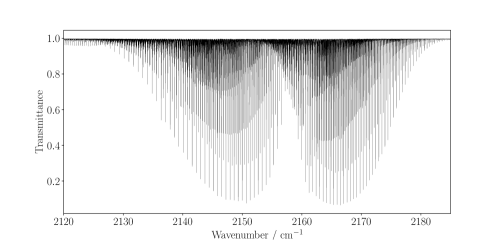
Figure 1: Experimental high-resolution spectrum of between 2120 and 2185
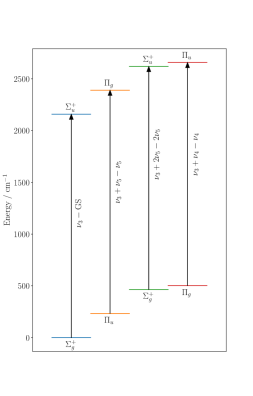
Figure 2: The four vibrational bands presented in this work: and Symmetries are labeled for each energy levels.
For the band, 201 lines have been assigned from to A few lines have been systematically removed from the fit if they were obviously blended with other lines, and decreased the quality of the fit. The average error defined as
where is the number of observations, and is the difference in between the observed and calculated position of line In our fit of the fundamental band For the hot band 114 lines have been assigned, from to with and are both states, meaning there are no doubling observed for those two bands. This is not the case for and which are respectively and states. As lines are blended for low (because the splitting is not big enough), we did not include lines with for and for while fitting positions. The evolution of the splitting as increases is illustrated in Fig. 10.
For we fitted 195 lines from to with For we fitted 323 lines from to with The fit residuals for the line positions of each band discussed are represented in Fig. 3a, 3b, 3c and 3d. Residuals are plotted against the upper level rotational quantum number to highlight potential non-zero higher-terms in the polynomial expansion of the energy states. The total average error (considering the four bands together) is and all the fit residuals are represented in Fig. 3e, where the x-axis is now the wavenumber in
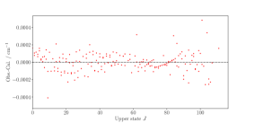
(a) Fit residuals for the band. 190 observations, average error:
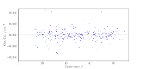
(b) Fit residuals for the band. 234 observations, average error:
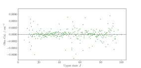
(c) Fit residuals for the band. 319 observations, average error:
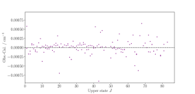
(d) Fit residuals for the band. 137 observations, average error:
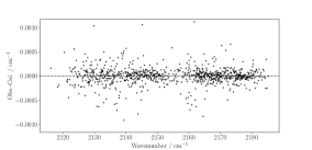
(e) Fit residuals for all four bands, plotted against wavenumber. 880 observations, average error:
Figure 3: Fit residuals for the line positions of the vibrational bands of with respect to the upper state rotational quantum number and wavenumber.
The spectroscopic parameters derived from the fit in positions are summarized in Table 3. The standard deviation is indicated in parentheses. No parentheses indicate that the value was fixed using values from [21].
|
|
|
|
|
|
|
|
|
|
|
|
|
|
|
|
|
|
Origin |
B |
D |
|
H |
|
L |
|
q |
|
qD |
|
qH |
|
qL |
|
| GS |
0 |
0.1570879982(2801) |
|
|
0 |
|
0 |
|
0 |
|
0 |
|
0 |
|
0 |
|
| |
|
0.1576278497(3905) |
|
|
|
|
0 |
|
|
|
|
|
0 |
|
0 |
|
| |
|
0.158166967(1048) |
|
|
|
|
|
|
0 |
|
0 |
|
0 |
|
0 |
|
| |
|
0.1574531178(2931) |
|
|
0 |
|
0 |
|
|
|
|
|
|
|
|
|
| |
2157.824256(34) |
0.1565544657(2892) |
|
|
|
|
|
|
0 |
|
0 |
|
0 |
|
0 |
|
| |
2389.736280(30) |
0.1570968635(3867) |
|
|
|
|
0 |
|
|
|
|
|
0 |
|
0 |
|
| |
2619.092571(39) |
0.157638754(1055) |
|
|
|
|
|
|
0 |
|
0 |
|
0 |
|
0 |
|
| |
2657.530013(67) |
0.1569204218(3257) |
|
|
|
|
|
|
|
|
|
|
|
|
|
|
Table 3: Derived parameters from the lines positions analysis in PGOPHER. Uncertainties are indicated in parentheses, in units of the last digits. rotational constant, centrifugal distortion, centrifugal distortion, centrifugal distortion, lambda-doubling constant, centrifugal distortion of centrifugal distortion of centrifugal distortion of values coming from [21], all values are in units of
4.2 Intensities
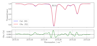
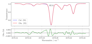
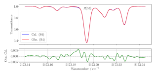
We restricted our intensity analysis to the band, as the cometary fluorescence model will focus only on this band. The fit was done using the MSFP (Multi-Spectrum Fitting Program), developed by Jean Vander Auwera at Université Libre de Bruxelles. This program takes as input the spectra recorded under different conditions, the total internal partition function of the considered species, and the linelists to be fitted. We measured the intensity and self-broadening coefficients of 147 lines of the band by fitting Voigt profiles. As an example, the line is represented for three different pressures (S2, S3, S4) in Fig. 4. We did not include lines known to be blended with absorption lines originating from the three hot bands discussed earlier because the measured lines intensity and broadening are overestimated in those cases. From the measurements and the intensity formula (equation 4), we have derived the band strength of in [3]). The first term in the Herman-Wallis correction was also derived, and we found The comparison between the measured intensities and the calculated intensities is represented in Fig. 9. The intensity fit has a root mean square deviation equal to 6.383%.
(a)
(b)
(c)
Figure 4: Simulation (in red) and observation (in blue) of the line of in the S2 (a), S3 (b), S4 (c)
spectra. Residuals are shown in green for each case.
5 Development of a cometary fluorescence model
5.1 Ground-state population and energy levels
From our analysis, we first computed the energy levels of cyanogen in the ground state. As a parent species, it is assumed that the initial population of is mainly in the ground state. This is because the temperature in the coma is very low (typically a few tens of kelvin), and the sublimation of the parent species from the nucleus to the coma does not excite the molecules to higher vibrational states. Moreover, in a first good approximation, collisions are negligible because the coma is an optically thin environment. The initial population distribution in the ground state follows:
and the initial fractional population is the ratio between and the total partition function at temperature
5.2 Branching ratio from the ground state to
The population of the upper state is determined using branching ratios, defined as:
which we develop as:
In absorption, corresponds to the branch, while corresponds to the branch. The populated level in the ground state is split to branch) or branch) level of the excited level, following usual selection rules for roto-vibrational transitions of linear molecules:
In our case, and GS being both states, and the branch is forbidden. The fractional population in the excited state is then:
As an example, the excited level is populated from the ground states and and
This is illustrated by green arrows in Fig. 5. Values for and up to at K are presented in Table 4.
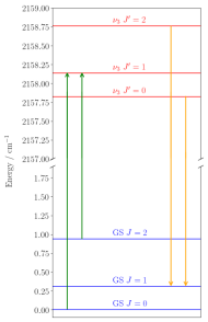
Figure 5: Schematic representation of the fluorescence process. The pumping from GS to is represented in green, and the pumping from to GS is represented in orange. The y-axis has been broken for clarification.
|
|
|
|
|
|
GS |
← |
|
← |
| J/J’ |
|
|
|
|
| 0 |
0.00 |
0.00600 |
2157.82 |
0.00297 |
| 1 |
0.31 |
0.00892 |
2158.14 |
0.01767 |
| 2 |
0.94 |
0.02921 |
2158.76 |
0.01446 |
| 3 |
1.89 |
0.01990 |
2159.70 |
0.03943 |
| 4 |
3.14 |
0.04936 |
2160.96 |
0.02446 |
| 5 |
4.71 |
0.02883 |
2162.52 |
0.05717 |
| 6 |
6.60 |
0.06455 |
2164.40 |
0.03202 |
| 7 |
8.80 |
0.03496 |
2166.59 |
0.06941 |
| 8 |
11.31 |
0.07370 |
2169.10 |
0.03662 |
| 9 |
14.14 |
0.03797 |
2171.91 |
0.07552 |
| 10 |
17.28 |
0.07668 |
2175.04 |
0.03817 |
| 11 |
20.74 |
0.03801 |
2178.49 |
0.07577 |
| 12 |
24.51 |
0.07414 |
2182.25 |
0.03699 |
| 13 |
28.59 |
0.03560 |
2186.32 |
0.07114 |
| 14 |
32.99 |
0.06738 |
2190.70 |
0.03371 |
| 15 |
37.70 |
0.03145 |
2195.40 |
0.06302 |
| 16 |
42.73 |
0.05793 |
2200.41 |
0.02907 |
| 17 |
48.07 |
0.02635 |
2205.73 |
0.05298 |
| 18 |
53.72 |
0.04734 |
2211.36 |
0.02384 |
| 19 |
59.69 |
0.02101 |
2217.31 |
0.04241 |
| 20 |
65.97 |
0.03687 |
2223.57 |
0.01864 |
← continues the cell to its left.
Table 4: Energy levels and fractional population of in the ground state (GS) and in the excited state, with K.
Finally, the population which falls back from the excited level to the level in the Ground State through the branch or branch is :
where is now defined as This unusual choice in spectroscopy (where is normally was made to stay consistent with equations 14 and 15. The corresponding emission factors are obtained by multiplying by the g-factor of the band (defined in equation 9):
5.3 Excitation rates
For the band, considering an excitation by the Sun at 1 au, photons a value 50% higher than the one reported in [3], despite reporting a similar band strength. We explain this difference by an underestimation of the vibrational partition function in [3], impacting the Einstein coefficient of the band and therefore the g-factor of the band (respectively equations 8 and 9). At 300 K, in [3], while we have and [12] have Excitation rates up to for K are presented in Table 5, and represented in Fig. 6.
|
|
|
|
|
|
| Line |
|
|
Line |
|
|
|
2151.3387 |
1.126 |
|
2158.1374 |
0.312 |
|
2151.6730 |
0.634 |
|
2158.4494 |
0.307 |
|
2152.0063 |
1.414 |
|
2158.7604 |
0.897 |
|
2152.3386 |
0.778 |
|
2159.0703 |
0.577 |
|
2152.6697 |
1.691 |
|
2159.3791 |
1.382 |
|
2152.9999 |
0.907 |
|
2159.6869 |
0.787 |
|
2153.3289 |
1.922 |
|
2159.9936 |
1.726 |
|
2153.6569 |
1.003 |
|
2160.2992 |
0.919 |
|
2153.9839 |
2.064 |
|
2160.6038 |
1.910 |
|
2154.3097 |
1.045 |
|
2160.9072 |
0.972 |
|
2154.6346 |
2.080 |
|
2161.2097 |
1.939 |
|
2154.9583 |
1.015 |
|
2161.5110 |
0.951 |
|
2155.2810 |
1.941 |
|
2161.8113 |
1.837 |
|
2155.6026 |
0.905 |
|
2162.1105 |
0.874 |
|
2155.9232 |
1.639 |
|
2162.4086 |
1.639 |
|
2156.2427 |
0.715 |
|
2162.7056 |
0.758 |
|
2156.5612 |
1.187 |
|
2163.0016 |
1.386 |
|
2156.8785 |
0.458 |
|
2163.2965 |
0.625 |
|
2157.1948 |
0.622 |
|
2163.5903 |
1.115 |
|
2157.5101 |
0.157 |
|
2163.8830 |
0.491 |
Table 5: Wavenumbers and excitation rates (g-factors, noted of 40 lines with calculated at K and considering a Sun illumination at 1 au. Excitation rates are expressed in photons The excitation rate of the whole band is photons
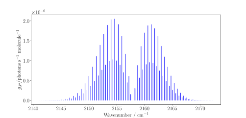
Figure 6: Emission factors of expressed in photons at T=50K. The values are the same as in Table 5.
6 Investigation in comet C/2022 E3 (ZTF)
6.1 Observations and data reduction
The Oort cloud comet C/2022 E3 (ZTF) was discovered on 2 March 2022 by the Zwicky Transient Facility. It reached perihelion in January 2023, at around 1.11 AU, with a peak magnitude of 5 ([4]). The comet was observed by JWST between 28 February and 4 March 2023, with au and 0.9 au ([22]). We investigated the JWST/NIRSPEC spectra obtained with the G395H/F290LP grating/filters configuration, covering the 2.87-5.27 µm range through the Integral Field Unit (IFU), with a field of view with the NRSIRS2RAPID readout and a 4-point dither [6]. The spectra were extracted with a 1.3” diameter. Third-level processed data were retrieved from the ESA JWST Science Archive1.
6.2 Haser model
The temperature of the coma was estimated by analyzing the intensity distribution of the band of the strongest emission feature in the spectrum. We assumed the gas to be in local thermodynamic equilibrium (LTE), and we expect the relative population levels to follow a Boltzmann law. From HITRAN database ([13]) and simulation of fluorescence spectrum in PGOPHER [28], we derived K. This is in agreement with the gas temperature derived from radio spectroscopy of the comet in early february by [2], where K. The band of and the simulation are represented in Fig. 7.
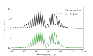
Figure 7: JWST/NIRSPEC spectrum of comet C/2022 E3 (ZTF) (in black) between 2320 and 2380 A first order background signal (due to the scattered light on the dust) has been removed, and the spectrum has then been normalized. The intensity distribution in the band enabled us to estimate the rotational temperature of as K. In green, a synthetic fluorescence spectrum at this rotational temperature, based on data from HITRAN [13] and convolved taking into account the resolving power of JWST/NIRSPEC is represented.
The production rate (in molecules is defined as
where is the geocentric distance (in meters), is the flux at the top of the atmosphere (in corrected for atmospheric transmittance at the Doppler-shifted line frequency, is the lifetime (in seconds) of the molecule, is the fluorescence efficiency (in photons per molecule of the emission line, is the energy (in Joules) of a photon with a wavenumber and is a geometric term representing the fraction of molecules sampled through the telescope aperture relative to the total number of molecules in the coma. We write the growth factor of the considered species, which is the ratio between the terminal production rate and the nucleus-centered production rate ([10]). In Eq. 25, and both depend on the heliocentric distance expressed in au). However, as (see Eq. 9) and their product is independent of the heliocentric distance.
To quantify an upper limit for in comet C/2022 E3 (ZTF), we used the Haser model ([17]), which describes the distribution of chemical species in the coma. It relies on the following hypothesis:
-
The cometary nucleus is assumed to be spherical, with a radius
-
Parent species are isotropically ejected away from the nucleus, with a constant velocity noted
-
The photodissociation of parent species is given by the law
where is the number of molecules at time and is the photodissociation lifetime of the corresponding molecule.
The density of parent species at a distance from the nucleus is given by
where is the production rate of the parent species (expressed in molecules and is the scalelength, defined as The column density of molecules, is obtained by integrating along the line of sight:
where we changed the variable of integration for such that and (the change of variables is illustrated in Fig. 11). We write the total number of molecules for a specific parent species observed through a circular aperture as
where we assumed that the aperture was centered on the nucleus. is the physical size at the comet given the geocentric distance with s in radian. The total number of molecules is obtained when in Eq. 30:
For a rectangular aperture of dimensions centered on the nucleus,
where Again, as the second term is much smaller than the first one, the total number of molecules is approximately:
The geometric factor in the production rate’s equation (Eq. 25) is then:
This factor depends on the slit’s dimensions the radius of the cometary nucleus (we assumed km), the geocentric distance the lifetime at the heliocentric distance and the ejection velocity of the parent species (we chose
The photodissociation rate of at 1 au was computed by [3], using vacuum ultraviolet spectra from [23]. This leads to a photodissociation lifetime at 1 au s, which is very close to the lifetime of acetylene at 1 au s), as reported by [9]
6.3 Upper limit for the production rate
We simulated synthetic spectra of up to to retrieve an upper limit (at level) in the spectrum of C/2022 E3 (ZTF). We assumed the rotational temperature of was equal to the rotational temperature derived with the band K). We convolved the emission lines using the resolving power of JWST/NIRSPEC, choosing a Gaussian profile for the convolution. The resolution of JWST/NIRSPEC in this configuration is too low to observe lines of individually, as its rotational constant is low As a comparison, the much larger rotational constant of CO [24]) leads to a much larger separation between two consecutive lines. This is illustrated in Fig. 8. We obtained molec. where this upper limit corresponds to the maximum production rate at which the total contribution of the band remains below the noise level in the JWST/NIRSPEC spectrum.
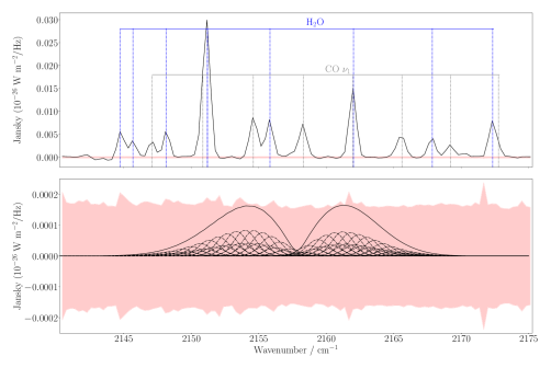
Figure 8: Top: JWST/NIRSPEC spectrum of comet C/2022 E3 (ZTF) between 2140 and 2175 Emission lines of CO and of are represented by alternated gray and blue lines, respectively. Bottom: Synthetic spectrum of (solid curve) calculated as the sum of lines (dashed lines) up to at K, convoluted by the JWST/NIRSPEC resolving power The flux error envelope is represented in pink in each plot.
6.4 Mixing ratio estimates
From three water lines with known g-factors at K (summarized in Table 6) ([11]), we estimated the production rate of water of C/2022 E3 (ZTF) on 01/03/23 as molec.
|
|
|
|
|
|
| Band assignment |
Line assignment |
Rest frequency |
g-Factors at 60K |
Measured flux |
|
| 100-010 |
|
2039.95 |
|
|
|
| 001-010 |
|
2137.37 |
|
|
|
| 001-010 |
|
2151.19 |
|
|
|
Table 6: Emission lines of water used to estimate the water production rate in comet C/2022 E3 (ZTF) on 01/03/23. g-Factors (from [11]) are expressed for and assuming an ortho to para ratio of 3.
We assumed a usual ortho to para ratio of 3, and a growth factor of 1.8. The derived value is very close to the mean production rate of water derived by [7] (reported in [20]) one month prior to JWST measurements, when au (post-perihelion): molec. Our upper limit on the mixing ratio of is This value is still higher than the abundances derived in situ in the coma of 67P [14]: = (1.24-1.74 au), and = in May 2015, at the same time of detection of ([26]).
6.5 Perspectives
The high value obtained for the mixing ratio is mainly due to the low fluorescence efficiencies of Despite this limiting factor, future observations may provide a more refined upper limit, particularly if a brighter comet is observed. A higher intrinsic brightness would improve the signal-to-noise ratio, making the detection of weaker spectral features more feasible. Additionally, advancements in telescope technology will contribute to reducing uncertainties. Instruments like METIS (Mid-Infrared ELT Imager and Spectrograph), planned for installation in 2028 on the 39-meter ESO Extremely Large Telescope (ELT) [5], will offer high-resolution spectroscopy in the L/M infrared windows. The combination of increased collecting area and improved spectral resolution could allow for better constraints on production rates, offering new opportunities to probe its presence in cometary atmospheres.
7 Conclusions
This study presents a new fluorescence model for the vibrational band of cyanogen offering a robust tool for analyzing its spectral characteristics in cometary environments. By combining high-resolution laboratory spectra with detailed theoretical modeling, we have, for the first time, derived line-by-line excitation rates for this molecule. The analysis of the band confirms that cyanogen’s fluorescence efficiency is low; however, future advancements, such as the METIS spectrometer on the ELT, are expected to significantly improve the detection and characterization of cyanogen in cometary spectra.
Cyanogen is the second molecule studied as part of the COSMIC project (COmputation and Spectroscopy of Molecules in the Infrared for Comets), following chloromethane [16]). Although the ESA/Rosetta mission led to the discovery of approximately 40 new molecules, molecular databases remain incomplete, lacking data on many key species needed to analyze trace elements in cometary spectra effectively. This work highlights the importance of continued laboratory spectroscopy efforts to expand these databases and enhance our understanding of cometary chemistry, and of the origins of our solar system.
A Additional figures
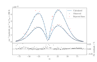
Figure 9: up Comparison between measured (dots) and calculated (blue solid lines) intensities of absorption lines with respect to m. Black points represent the 147 lines that were used to derive the band strength and the Herman-Wallis correction. We also represented the rejected lines in red: they correspond to lines blended with at least one line originating from a hot band. Error bars are displayed for each point, but are too small to be seen in most of the cases. bottom Fit residuals, expressed as the relative difference ((Obs.-Cal.)/Cal.), showing deviations between observed and calculated intensities.
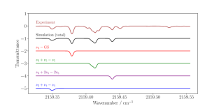
(a) Comparison between the calculated and experimental spectrum in the region 2159.33-2159.56 The lines (in green) and the lines (in blue) are blended.
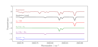
(b) Comparison between the calculated and experimental spectrum in the region 2163.69-2163.92 The lines (in green) and the lines (in blue) are separating.
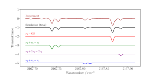
(c) Comparison between the calculated and experimental spectrum in the region 2167.69-2167.92 The lines (in green) and the lines (in blue) are well separated.
Figure 10: Three regions in the branch with increasing rotational quantum number (in respect to each band) from (a) to (c). The splitting of and is getting stronger as is increasing. Some absorption lines coming from hot bands not taken into account in this work can be observed while comparing the experimental spectrum (in brown) with the total simulation (in black). An arbitrary Gaussian profile and relative intensities have been chosen to calculate the spectra in PGOPHER.
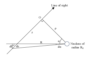
Figure 11: Variables used to derive the integral in equation 29. and This leads to
References
[1] Altwegg, K., Balsiger, H., & Fuselier, S. A. 2019, Annual Review of Astronomy and Astrophysics, 57, 113–155
[2] Biver, N., Bockelée-Morvan, D., Handzlik, B., et al. 2024, Astronomy and Astrophysics, 690, A271
[3] Bockelee-Morvan, D. & Crovisier, J. 1985, Astronomy and Astrophysics, 151, 90
[4] Bolin, B. T., Masci, F. J., Ip, W. H., et al. 2022, Minor Planet Electronic Circulars, 2022-F13
[5] Brandl, B. R., Absil, O., Agócs, T., et al. 2018, in Society of Photo-Optical Instrumentation Engineers (SPIE) Conference Series, Vol. 10702, Ground-based and Airborne Instrumentation for Astronomy VII, ed. C. J. Evans, L. Simard, & H. Takami, 107021U
[6] Böker, T., Beck, T. L., Birkmann, S. M., et al. 2023, Publications of the Astronomical Society of the Pacific, 135, 038001
[7] Combi, M., Mäkinen, T., Bertaux, J.-L., Quemerais, E., & Ferron, S. 2023, in AAS/Division for Planetary Sciences Meeting Abstracts, Vol. 55, AAS/Division for Planetary Sciences Meeting Abstracts #55, 322.04
[8] Crovisier, J. 1984, Astronomy and Astrophysics, 130, 361
[9] Crovisier, J. & Encrenaz, T. 1983, Astronomy and Astrophysics, 126, 170
[10] Dello Russo, N., DiSanti, M. A., Mumma, M. J., Magee-Sauer, K., & Rettig, T. W. 1998, icarus, 135, 377
[11] Dello Russo, N., Mumma, M. J., DiSanti, M. A., et al. 2000, Icarus, 143, 324
[12] Fayt, A., Jolly, A., Benilan, Y., et al. 2012, Journal of Quantitative Spectroscopy and Radiative Transfer, 113, 1195, three Leaders in Spectroscopy
[13] Gordon, I., Rothman, L., Hargreaves, R., et al. 2022, Journal of Quantitative Spectroscopy and Radiative Transfer, 277, 107949
[14] Hänni, N., Altwegg, K., Balsiger, H., et al. 2021, Astronomy and Astrophysics, 647, A22
[15] Hänni, N., Altwegg, K., Pestoni, B., et al. 2020, Monthly Notices of the Royal Astronomical Society, 498, 2239–2248
[16] Hardy, P., Richard, C., Boudon, V., et al. 2023, Journal of Quantitative Spectroscopy and Radiative Transfer, 311, 108779
[17] Haser, L. 1957, Bulletins de l’Académie Royale de Belgique, 43, 740
[18] Herzberg, G. 1950, Molecular Spectra and Molecular Structure: I. Spectra of Diatomic Molecules (New York: Van Nostrand Reinhold)
[19] Kunde, V. G., Aikin, A. C., Hanel, R. A., et al. 1981, Nature, 292, 686–688
[20] Li, J., Shi, J., Ma, Y., & Sun, J. 2025, The Astronomical Journal, 169, 126
[21] Maki, A. G. 2011, Journal of Molecular Spectroscopy, 269, 166
[22] Milam, S. N., Roth, N. X., Villanueva, G. L., et al. 2023, in LPI Contributions, Vol. 2851, Asteroids, Comets, Meteors Conference, 2163
[23] Nuth, J. A. & Glicker, S. 1982, Journal of Quantitative Spectroscopy and Radiative Transfer, 28, 223
[24] Rank, D., Pierre, A., & Wiggins, T. 1965, Journal of Molecular Spectroscopy, 18, 418
[25] Rothman, L. S. & Young, L. D. G. 1981, Journal of Quantitative Spectroscopy and Radiative Transfer, 25, 505
[26] Rubin, M., Altwegg, K., Balsiger, H., et al. 2019, Monthly Notices of the Royal Astronomical Society, 489, 594
[27] Russo, N. D., Mumma, M. J., DiSanti, M. A., Magee-Sauer, K., & Novak, R. 2001, Icarus, 153, 162
[28] Western, C. M. 2017, Journal of Quantitative Spectroscopy and Radiative Transfer, 186, 221, satellite Remote Sensing and Spectroscopy: Joint ACE-Odin Meeting, October 2015
1https://jwst.esac.esa.int/archive/
About this conversion
“A Refined Cometary Fluorescence Model for the ν₃ Vibrational Band of Cyanogen: Application to JWST/NIRSPEC Spectrum” by P. Hardy, P. Rousselot, C. Richard, V. Boudon, X. Landsheere, A. Voute, L. Manceron, F. Kwabia Tchana. Original arXiv submission, 2503.18128v2. Shared under Creative Commons Attribution 4.0 International, as identified by the exact-version arXiv record.
Linneon LLC converted the original LaTeX submission to continuous Markdown and HTML using LEC on October 14, 2026. Pagination and page furniture are removed; tables, notes and figures are arranged for continuous reading. HTML mathematics uses MathJax. These reading copies are not the official publication and do not imply endorsement by the authors, their institutions or arXiv. Original notices are retained. Dates generated by the source may reflect recompilation.